Wsrtjtyk

measure of covariance of components of a random vector

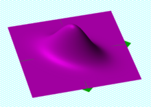
A bivariate Gaussian probability density function centered at (0, 0), with covariance matrix given by

{displaystyle {begin{bmatrix}1&0.5\0.5&1end{bmatrix}}}

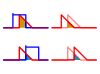
Sample points from a bivariate Gaussian distribution with a standard deviation of 3 in roughly the lower left-upper right direction and of 1 in the orthogonal direction. Because the x and y components co-vary, the variances of

x

and

y

do not fully describe the distribution. A

2times 2

covariance matrix is needed; the directions of the arrows correspond to the eigenvectors of this covariance matrix and their lengths to the square roots of the eigenvalues.

In probability theory and statistics, a covariance matrix, also known as auto-covariance matrix, dispersion matrix, variance matrix, or variance–covariance matrix, is a matrix whose element in the i, j position is the covariance between the i-th and j-th elements of a random vector. A random vector is a random variable with multiple dimensions. Each element of the vector is a scalar random variable. Each element has either a finite number of observed empirical values or a finite or infinite number of potential values. The potential values are specified by a theoretical joint probability distribution.

Intuitively, the covariance matrix generalizes the notion of variance to multiple dimensions. As an example, the variation in a collection of random points in two-dimensional space cannot be characterized fully by a single number, nor would the variances in the $x$ and $y$ directions contain all of the necessary information; a $2times 2$ matrix would be necessary to fully characterize the two-dimensional variation.

Because the covariance of the i-th random variable with itself is simply that random variable's variance, each element on the principal diagonal of the covariance matrix is the variance of one of the random variables. Because the covariance of the i-th random variable with the j-th one is the same thing as the covariance of the j-th random variable with the i-th random variable, every covariance matrix is symmetric. Also, every covariance matrix is positive semi-definite.

The auto-covariance matrix of a random vector $mathbf {X}$ is typically denoted by ${displaystyle operatorname {K} _{mathbf {X} mathbf {X} }}$ or $Sigma$ .

Definition

Throughout this article, boldfaced unsubscripted $mathbf {X}$ and $mathbf {Y}$ are used to refer to random vectors, and unboldfaced subscripted $X_{i}$ and $Y_{i}$ are used to refer to scalar random variables.

If the entries in the column vector

{displaystyle mathbf {X} =(X_{1},X_{2},...,X_{n})^{mathrm {T} }}

are random variables, each with finite variance and expected value, then the covariance matrix ${displaystyle operatorname {K} _{mathbf {X} mathbf {X} }}$ is the matrix whose $(i,j)$ entry is the covariance^[1]^{:p. 177}

{displaystyle operatorname {K} _{X_{i}X_{j}}=operatorname {cov} [X_{i},X_{j}]=operatorname {E} [(X_{i}-operatorname {E} [X_{i}])(X_{j}-operatorname {E} [X_{j}])]}

where the operator $operatorname {E}$ denotes the expected value (mean) of its argument.

In other words,

{displaystyle operatorname {K} _{mathbf {X} mathbf {X} }={begin{bmatrix}mathrm {E} [(X_{1}-operatorname {E} [X_{1}])(X_{1}-operatorname {E} [X_{1}])]&mathrm {E} [(X_{1}-operatorname {E} [X_{1}])(X_{2}-operatorname {E} [X_{2}])]&cdots &mathrm {E} [(X_{1}-operatorname {E} [X_{1}])(X_{n}-operatorname {E} [X_{n}])]\\mathrm {E} [(X_{2}-operatorname {E} [X_{2}])(X_{1}-operatorname {E} [X_{1}])]&mathrm {E} [(X_{2}-operatorname {E} [X_{2}])(X_{2}-operatorname {E} [X_{2}])]&cdots &mathrm {E} [(X_{2}-operatorname {E} [X_{2}])(X_{n}-operatorname {E} [X_{n}])]\\vdots &vdots &ddots &vdots \\mathrm {E} [(X_{n}-operatorname {E} [X_{n}])(X_{1}-operatorname {E} [X_{1}])]&mathrm {E} [(X_{n}-operatorname {E} [X_{n}])(X_{2}-operatorname {E} [X_{2}])]&cdots &mathrm {E} [(X_{n}-operatorname {E} [X_{n}])(X_{n}-operatorname {E} [X_{n}])]end{bmatrix}}}

The definition above is equivalent to the matrix equality

${displaystyle operatorname {K} _{mathbf {X} mathbf {X} }=operatorname {cov} [mathbf {X} ,mathbf {X} ]=operatorname {E} [(mathbf {X} -mathbf {mu _{X}} )(mathbf {X} -mathbf {mu _{X}} )^{rm {T}}]=operatorname {E} [mathbf {X} mathbf {X} ^{T}]-mathbf {mu _{X}} mathbf {mu _{X}} ^{T}}$

(Eq.1)

where ${displaystyle mathbf {mu _{X}} =operatorname {E} [mathbf {X} ]}$ .

Generalization of the variance

This form (Eq.1) can be seen as a generalization of the scalar-valued variance to higher dimensions. Recall that for a scalar-valued random variable $X$

{displaystyle sigma _{X}^{2}=operatorname {var} (X)=operatorname {E} [(X-operatorname {E} [X])^{2}]=operatorname {E} [(X-operatorname {E} [X])cdot (X-operatorname {E} [X])].}

Indeed, the entries on the diagonal of the auto-covariance matrix ${displaystyle operatorname {K} _{mathbf {X} mathbf {X} }}$ are the variances of each element of the vector $mathbf {X}$ .

Conflicting nomenclatures and notations

Nomenclatures differ. Some statisticians, following the probabilist William Feller in his two-volume book An Introduction to Probability Theory and Its Applications,^[2] call the matrix ${displaystyle operatorname {K} _{mathbf {X} mathbf {X} }}$ the variance of the random vector $mathbf {X}$ , because it is the natural generalization to higher dimensions of the 1-dimensional variance. Others call it the covariance matrix, because it is the matrix of covariances between the scalar components of the vector $mathbf {X}$ .

{displaystyle operatorname {var} (mathbf {X} )=operatorname {cov} (mathbf {X} )=operatorname {E} left[(mathbf {X} -operatorname {E} [mathbf {X} ])(mathbf {X} -operatorname {E} [mathbf {X} ])^{rm {T}}right].}

Both forms are quite standard, and there is no ambiguity between them. The matrix ${displaystyle operatorname {K} _{mathbf {X} mathbf {X} }}$ is also often called the variance-covariance matrix, since the diagonal terms are in fact variances.

By comparison, the notation for the cross-covariance matrix between two vectors is

{displaystyle operatorname {cov} (mathbf {X} ,mathbf {Y} )=operatorname {K} _{mathbf {X} mathbf {Y} }=operatorname {E} left[(mathbf {X} -operatorname {E} [mathbf {X} ])(mathbf {Y} -operatorname {E} [mathbf {Y} ])^{rm {T}}right].}

Properties

Relation to the correlation matrix

The auto-covariance matrix ${displaystyle operatorname {K} _{mathbf {X} mathbf {X} }}$ is related to the autocorrelation matrix ${displaystyle operatorname {R} _{mathbf {X} mathbf {X} }}$ by

{displaystyle operatorname {K} _{mathbf {X} mathbf {X} }=operatorname {E} [(mathbf {X} -operatorname {E} [mathbf {X} ])(mathbf {X} -operatorname {E} [mathbf {X} ])^{rm {T}}]=operatorname {R} _{mathbf {X} mathbf {X} }-operatorname {E} [mathbf {X} ]operatorname {E} [mathbf {X} ]^{rm {T}}}

where the autocorrelation matrix is defined as ${displaystyle operatorname {R} _{mathbf {X} mathbf {X} }=operatorname {E} [mathbf {X} mathbf {X} ^{rm {T}}]}$ .

Relation to the matrix of correlation coefficients

An entity closely related to the covariance matrix is the matrix of Pearson product-moment correlation coefficients between each of the random variables in the random vector $mathbf {X}$ , which can be written as

{displaystyle operatorname {corr} (mathbf {X} )={big (}operatorname {diag} (operatorname {K} _{mathbf {X} mathbf {X} }){big )}^{-{frac {1}{2}}},operatorname {K} _{mathbf {X} mathbf {X} },{big (}operatorname {diag} (operatorname {K} _{mathbf {X} mathbf {X} }){big )}^{-{frac {1}{2}}},}

where ${displaystyle operatorname {diag} (operatorname {K} _{mathbf {X} mathbf {X} })}$ is the matrix of the diagonal elements of ${displaystyle operatorname {K} _{mathbf {X} mathbf {X} }}$ (i.e., a diagonal matrix of the variances of $X_{i}$ for $i=1,dots ,n$ ).

Equivalently, the correlation matrix can be seen as the covariance matrix of the standardized random variables $X_{i}/sigma (X_{i})$ for $i=1,dots ,n$ .

{displaystyle operatorname {corr} (mathbf {X} )={begin{bmatrix}1&{frac {operatorname {E} [(X_{1}-mu _{1})(X_{2}-mu _{2})]}{sigma (X_{1})sigma (X_{2})}}&cdots &{frac {operatorname {E} [(X_{1}-mu _{1})(X_{n}-mu _{n})]}{sigma (X_{1})sigma (X_{n})}}\\{frac {operatorname {E} [(X_{2}-mu _{2})(X_{1}-mu _{1})]}{sigma (X_{2})sigma (X_{1})}}&1&cdots &{frac {operatorname {E} [(X_{2}-mu _{2})(X_{n}-mu _{n})]}{sigma (X_{2})sigma (X_{n})}}\\vdots &vdots &ddots &vdots \\{frac {operatorname {E} [(X_{n}-mu _{n})(X_{1}-mu _{1})]}{sigma (X_{n})sigma (X_{1})}}&{frac {operatorname {E} [(X_{n}-mu _{n})(X_{2}-mu _{2})]}{sigma (X_{n})sigma (X_{2})}}&cdots &1end{bmatrix}}.}

Each element on the principal diagonal of a correlation matrix is the correlation of a random variable with itself, which always equals 1. Each off-diagonal element is between −1 and +1 inclusive.

Inverse of the covariance matrix

The inverse of this matrix, ${displaystyle operatorname {K} _{mathbf {X} mathbf {X} }^{-1}}$ , if it exists, is the inverse covariance matrix, also known as the concentration matrix or precision matrix.^[3]

Basic properties

For ${displaystyle operatorname {K} _{mathbf {X} mathbf {X} }=operatorname {var} (mathbf {X} )=operatorname {E} left[left(mathbf {X} -operatorname {E} [mathbf {X} ]right)left(mathbf {X} -operatorname {E} [mathbf {X} ]right)^{rm {T}}right]}$ and ${displaystyle mathbf {mu _{X}} =operatorname {E} ({textbf {X}})}$ , where ${displaystyle mathbf {X} =(X_{1},ldots ,X_{n})}$ is a $n$ -dimensional random variable, the following basic properties apply:^[4]

${displaystyle operatorname {K} _{mathbf {X} mathbf {X} }=operatorname {E} (mathbf {XX^{rm {T}}} )-mathbf {mu _{X}} mathbf {mu _{X}} ^{rm {T}}}$

${displaystyle operatorname {K} _{mathbf {X} mathbf {X} },}$ is positive-semidefinite, i.e. ${displaystyle mathbf {a} ^{T}Sigma mathbf {a} geq 0quad {text{for all }}mathbf {a} in mathbb {R} ^{n}}$

${displaystyle operatorname {K} _{mathbf {X} mathbf {X} },}$ is symmetric, i.e. ${displaystyle operatorname {K} _{mathbf {X} mathbf {X} }^{rm {T}}=operatorname {K} _{mathbf {X} mathbf {X} }}$

For any constant (i.e. non-random) $mtimes n$ matrix $mathbf {A}$ and constant $mtimes 1$ vector $mathbf {a}$ , one has ${displaystyle operatorname {var} (mathbf {AX} +mathbf {a} )=mathbf {A} ,operatorname {var} (mathbf {X} ),mathbf {A} ^{rm {T}}}$

If $mathbf {Y}$ is another random vector with the same dimension as $mathbf {X}$ , then ${displaystyle operatorname {var} (mathbf {X} +mathbf {Y} )=operatorname {var} (mathbf {X} )+operatorname {cov} (mathbf {X} ,mathbf {Y} )+operatorname {cov} (mathbf {Y} ,mathbf {X} )+operatorname {var} (mathbf {Y} )}$ where ${displaystyle operatorname {cov} (mathbf {X} ,mathbf {Y} )}$ is the cross-covariance matrix of $mathbf {X}$ and $mathbf {Y}$ .

Block matrices

The joint mean ${displaystyle mathbf {mu } _{X,Y}}$ and joint covariance matrix ${boldsymbol {Sigma }}_{X,Y}$ of $mathbf {X}$ and $mathbf {Y}$ can be written in block form

{boldsymbol {mu }}_{X,Y}={begin{bmatrix}{boldsymbol {mu }}_{X}\{boldsymbol {mu }}_{Y}end{bmatrix}},qquad {boldsymbol {Sigma }}_{X,Y}={begin{bmatrix}{boldsymbol {Sigma }}_{mathit {XX}}&{boldsymbol {Sigma }}_{mathit {XY}}\{boldsymbol {Sigma }}_{mathit {YX}}&{boldsymbol {Sigma }}_{mathit {YY}}end{bmatrix}}

where ${displaystyle {boldsymbol {Sigma }}_{XX}=operatorname {var} ({boldsymbol {X}}),{boldsymbol {Sigma }}_{YY}=operatorname {var} ({boldsymbol {Y}}),}$ and ${displaystyle {boldsymbol {Sigma }}_{XY}={boldsymbol {Sigma }}_{mathit {YX}}^{T}=operatorname {cov} ({boldsymbol {X}},{boldsymbol {Y}})}$ .

${boldsymbol {Sigma }}_{XX}$ and ${boldsymbol {Sigma }}_{YY}$ can be identified as the variance matrices of the marginal distributions for ${boldsymbol {X}}$ and ${boldsymbol {Y}}$ respectively.

If ${boldsymbol {X}}$ and ${boldsymbol {Y}}$ are jointly normally distributed,

{displaystyle {boldsymbol {X}},{boldsymbol {Y}}sim {mathcal {N}}({boldsymbol {mu }}_{X,Y},{boldsymbol {Sigma }}_{X,Y}),}

then the conditional distribution for ${boldsymbol {Y}}$ given ${boldsymbol {X}}$ is given by

{displaystyle {boldsymbol {Y}}mid {boldsymbol {X}}sim {mathcal {N}}({boldsymbol {mu }}_{Y|X},{boldsymbol {Sigma }}_{Ymid X}),}

^[5]

defined by conditional mean

{displaystyle {boldsymbol {mu }}_{Ymid X}={boldsymbol {mu }}_{Y}+{boldsymbol {Sigma }}_{YX}{boldsymbol {Sigma }}_{XX}^{-1}left(mathbf {x} -{boldsymbol {mu }}_{X}right)}

and conditional variance

{displaystyle {boldsymbol {Sigma }}_{Ymid X}={boldsymbol {Sigma }}_{YY}-{boldsymbol {Sigma }}_{mathit {YX}}{boldsymbol {Sigma }}_{mathit {XX}}^{-1}{boldsymbol {Sigma }}_{mathit {XY}}.}

The matrix ${displaystyle {boldsymbol {Sigma }}_{YX}{boldsymbol {Sigma }}_{XX}^{-1}}$ is known as the matrix of regression coefficients, while in linear algebra ${displaystyle {boldsymbol {Sigma }}_{Ymid X}}$ is the Schur complement of ${boldsymbol {Sigma }}_{XX}$ in ${boldsymbol {Sigma }}_{X,Y}$ .

The matrix of regression coefficients may often be given in transpose form, ${displaystyle {boldsymbol {Sigma }}_{XX}^{-1}{boldsymbol {Sigma }}_{XY}}$ , suitable for post-multiplying a row vector of explanatory variables x^T rather than pre-multiplying a column vector x. In this form they correspond to the coefficients obtained by inverting the matrix of the normal equations of ordinary least squares (OLS).

Covariance matrix as a parameter of a distribution

If a vector of n possibly correlated random variables is jointly normally distributed, or more generally elliptically distributed, then its probability density function can be expressed in terms of the covariance matrix.^[6]

Covariance matrix as a linear operator

Applied to one vector, the covariance matrix maps a linear combination c of the random variables X onto a vector of covariances with those variables: ${displaystyle mathbf {c} ^{rm {T}}Sigma =operatorname {cov} (mathbf {c} ^{rm {T}}mathbf {X} ,mathbf {X} )}$ . Treated as a bilinear form, it yields the covariance between the two linear combinations: ${displaystyle mathbf {d} ^{rm {T}}Sigma mathbf {c} =operatorname {cov} (mathbf {d} ^{rm {T}}mathbf {X} ,mathbf {c} ^{rm {T}}mathbf {X} )}$ . The variance of a linear combination is then ${displaystyle mathbf {c} ^{rm {T}}Sigma mathbf {c} }$ , its covariance with itself.

Similarly, the (pseudo-)inverse covariance matrix provides an inner product ${displaystyle langle c-mu |Sigma ^{+}|c-mu rangle }$ , which induces the Mahalanobis distance, a measure of the "unlikelihood" of c.^{[citation needed]}

Which matrices are covariance matrices?

From the identity just above, let $mathbf {b}$ be a $(ptimes 1)$ real-valued vector, then

operatorname {var} (mathbf {b} ^{rm {T}}mathbf {X} )=mathbf {b} ^{rm {T}}operatorname {var} (mathbf {X} )mathbf {b} ,,

which must always be nonnegative, since it is the variance of a real-valued random variable. A covariance matrix is always a positive-semidefinite matrix, since

{displaystyle {begin{aligned}&w^{rm {T}}operatorname {E} left[(mathbf {X} -operatorname {E} [mathbf {X} ])(mathbf {X} -operatorname {E} [mathbf {X} ])^{rm {T}}right]w=operatorname {E} left[w^{rm {T}}(mathbf {X} -operatorname {E} [mathbf {X} ])(mathbf {X} -operatorname {E} [mathbf {X} ])^{rm {T}}wright]\[5pt]={}&operatorname {E} {big [}{big (}w^{rm {T}}(mathbf {X} -operatorname {E} [mathbf {X} ]){big )}^{2}{big ]}geq 0quad {text{since }}w^{rm {T}}(mathbf {X} -operatorname {E} [mathbf {X} ]){text{ is a scalar}}.end{aligned}}}

Conversely, every symmetric positive semi-definite matrix is a covariance matrix. To see this, suppose $M$ is a $ptimes p$ positive-semidefinite matrix. From the finite-dimensional case of the spectral theorem, it follows that $M$ has a nonnegative symmetric square root, which can be denoted by M^1/2. Let $mathbf {X}$ be any $ptimes 1$ column vector-valued random variable whose covariance matrix is the $ptimes p$ identity matrix. Then

{displaystyle operatorname {var} (mathbf {M} ^{1/2}mathbf {X} )=mathbf {M} ^{1/2},operatorname {var} (mathbf {X} ),mathbf {M} ^{1/2}=mathbf {M} .}

Complex random vectors

Covariance matrix

The variance of a complex scalar-valued random variable with expected value $mu$ is conventionally defined using complex conjugation:

{displaystyle operatorname {var} (Z)=operatorname {E} left[(Z-mu _{Z}){overline {(Z-mu _{Z})}}right],}

where the complex conjugate of a complex number $z$ is denoted ${overline {z}}$ ; thus the variance of a complex random variable is a real number.

If ${displaystyle mathbf {Z} =(Z_{1},ldots ,Z_{n})^{mathrm {T} }}$ is a column vector of complex-valued random variables, then the conjugate transpose is formed by both transposing and conjugating. In the following expression, the product of a vector with its conjugate transpose results in a square matrix called the covariance matrix, as its expectation:^[7]^{:p. 293}

{displaystyle operatorname {K} _{mathbf {Z} mathbf {Z} }=operatorname {cov} [mathbf {Z} ,mathbf {Z} ]=operatorname {E} left[(mathbf {Z} -mathbf {mu _{Z}} )(mathbf {Z} -mathbf {mu _{Z}} )^{mathrm {H} }right]}

,

where ${}^{mathrm {H} }$ denotes the conjugate transpose, which is applicable to the scalar case, since the transpose of a scalar is still a scalar. The matrix so obtained will be Hermitian positive-semidefinite,^[8] with real numbers in the main diagonal and complex numbers off-diagonal.

Pseudo-covariance matrix

For complex random vectors, another kind of second central moment, the pseudo-covariance matrix (also called relation matrix) is defined as follows. In contrast to the covariance matrix defined above Hermitian transposition gets replaced by transposition in the definition.

{displaystyle operatorname {J} _{mathbf {Z} mathbf {Z} }=operatorname {cov} [mathbf {Z} ,{overline {mathbf {Z} }}]=operatorname {E} left[(mathbf {Z} -mathbf {mu _{Z}} )(mathbf {Z} -mathbf {mu _{Z}} )^{mathrm {T} }right]}

Properties

The covariance matrix is a Hermitian matrix, i.e. ${displaystyle operatorname {K} _{mathbf {Z} mathbf {Z} }^{mathrm {H} }=operatorname {K} _{mathbf {Z} mathbf {Z} }}$ .^[1]^{:p. 179}

The diagonal elements of the covariance matrix are real.^[1]^{:p. 179}

Estimation

If $mathbf {M} _{mathbf {X} }$ and $mathbf {M} _{mathbf {Y} }$ are centred data matrices of dimension $ntimes p$ and ${displaystyle ntimes q}$ respectively, i.e. with n rows of observations of p and q columns of variables, from which the column means have been subtracted, then, if the column means were estimated from the data, sample correlation matrices $mathbf {Q} _{mathbf {X} }$ and $mathbf {Q} _{mathbf {XY} }$ can be defined to be

{displaystyle mathbf {Q} _{mathbf {X} }={frac {1}{n-1}}mathbf {M} _{mathbf {X} }^{rm {T}}mathbf {M} _{mathbf {X} },qquad mathbf {Q} _{mathbf {XY} }={frac {1}{n-1}}mathbf {M} _{mathbf {X} }^{rm {T}}mathbf {M} _{mathbf {Y} }}

or, if the column means were known a priori,

{displaystyle mathbf {Q} _{mathbf {X} }={frac {1}{n}}mathbf {M} _{mathbf {X} }^{rm {T}}mathbf {M} _{mathbf {X} },qquad mathbf {Q} _{mathbf {XY} }={frac {1}{n}}mathbf {M} _{mathbf {X} }^{rm {T}}mathbf {M} _{mathbf {Y} }.}

These empirical sample correlation matrices are the most straightforward and most often used estimators for the correlation matrices, but other estimators also exist, including regularised or shrinkage estimators, which may have better properties.

Applications

The covariance matrix is a useful tool in many different areas. From it a transformation matrix can be derived, called a whitening transformation, that allows one to completely decorrelate the data^{[citation needed]} or, from a different point of view, to find an optimal basis for representing the data in a compact way^{[citation needed]} (see Rayleigh quotient for a formal proof and additional properties of covariance matrices).
This is called principal component analysis (PCA) and the Karhunen–Loève transform (KL-transform).

The covariance matrix plays a key role in financial economics, especially in portfolio theory and its mutual fund separation theorem and in the capital asset pricing model. The matrix of covariances among various assets' returns is used to determine, under certain assumptions, the relative amounts of different assets that investors should (in a normative analysis) or are predicted to (in a positive analysis) choose to hold in a context of diversification.

References

^ ^a^b^c Park,Kun Il (2018). Fundamentals of Probability and Stochastic Processes with Applications to Communications. Springer. ISBN 978-3-319-68074-3..mw-parser-output cite.citation{font-style:inherit}.mw-parser-output .citation q{quotes:"""""""'""'"}.mw-parser-output .citation .cs1-lock-free a{background:url("//upload.wikimedia.org/wikipedia/commons/thumb/6/65/Lock-green.svg/9px-Lock-green.svg.png")no-repeat;background-position:right .1em center}.mw-parser-output .citation .cs1-lock-limited a,.mw-parser-output .citation .cs1-lock-registration a{background:url("//upload.wikimedia.org/wikipedia/commons/thumb/d/d6/Lock-gray-alt-2.svg/9px-Lock-gray-alt-2.svg.png")no-repeat;background-position:right .1em center}.mw-parser-output .citation .cs1-lock-subscription a{background:url("//upload.wikimedia.org/wikipedia/commons/thumb/a/aa/Lock-red-alt-2.svg/9px-Lock-red-alt-2.svg.png")no-repeat;background-position:right .1em center}.mw-parser-output .cs1-subscription,.mw-parser-output .cs1-registration{color:#555}.mw-parser-output .cs1-subscription span,.mw-parser-output .cs1-registration span{border-bottom:1px dotted;cursor:help}.mw-parser-output .cs1-ws-icon a{background:url("//upload.wikimedia.org/wikipedia/commons/thumb/4/4c/Wikisource-logo.svg/12px-Wikisource-logo.svg.png")no-repeat;background-position:right .1em center}.mw-parser-output code.cs1-code{color:inherit;background:inherit;border:inherit;padding:inherit}.mw-parser-output .cs1-hidden-error{display:none;font-size:100%}.mw-parser-output .cs1-visible-error{font-size:100%}.mw-parser-output .cs1-maint{display:none;color:#33aa33;margin-left:0.3em}.mw-parser-output .cs1-subscription,.mw-parser-output .cs1-registration,.mw-parser-output .cs1-format{font-size:95%}.mw-parser-output .cs1-kern-left,.mw-parser-output .cs1-kern-wl-left{padding-left:0.2em}.mw-parser-output .cs1-kern-right,.mw-parser-output .cs1-kern-wl-right{padding-right:0.2em}

^ William Feller (1971). An introduction to probability theory and its applications. Wiley. ISBN 978-0-471-25709-7. Retrieved 10 August 2012.

^ Wasserman, Larry (2004). All of Statistics: A Concise Course in Statistical Inference. ISBN 0-387-40272-1.

^ Taboga, Marco (2010). "Lectures on probability theory and mathematical statistics".

^ Eaton, Morris L. (1983). Multivariate Statistics: a Vector Space Approach. John Wiley and Sons. pp. 116–117. ISBN 0-471-02776-6.

^ Frahm, G.; Junker, M.; Szimayer, A. (2003). "Elliptical copulas: Applicability and limitations". Statistics & Probability Letters. 63 (3): 275–286. doi:10.1016/S0167-7152(03)00092-0.

^ Lapidoth, Amos (2009). A Foundation in Digital Communication. Cambridge University Press. ISBN 978-0-521-19395-5.

^ Brookes, Mike. "The Matrix Reference Manual".

v t e Matrix classes
Explicitly constrained entries	(0,1) Alternant Anti-diagonal Anti-Hermitian Anti-symmetric Arrowhead Band Bidiagonal Binary Bisymmetric Block-diagonal Block Block tridiagonal Boolean Cauchy Centrosymmetric Conference Complex Hadamard Copositive Diagonally dominant Diagonal Discrete Fourier Transform Elementary Equivalent Frobenius Generalized permutation Hadamard Hankel Hermitian Hessenberg Hollow Integer Logical Markov Metzler Monomial Moore Nonnegative Partitioned Parisi Pentadiagonal Permutation Persymmetric Polynomial Positive Quaternionic Sign Signature Skew-Hermitian Skew-symmetric Skyline Sparse Sylvester Symmetric Toeplitz Triangular Tridiagonal Unitary Vandermonde Walsh Z
Constant	Exchange Hilbert Identity Lehmer Of ones Pascal Pauli Redheffer Shift Zero
Conditions on eigenvalues or eigenvectors	Companion Convergent Defective Diagonalizable Hurwitz Positive-definite Stability Stieltjes
Satisfying conditions on products or inverses	Congruent Idempotent or Projection Invertible Involutory Nilpotent Normal Orthogonal Orthonormal Singular Unimodular Unipotent Totally unimodular Weighing
With specific applications	Adjugate Alternating sign Augmented Bézout Carleman Cartan Circulant Cofactor Commutation Coxeter Derogatory Distance Duplication Elimination Euclidean distance Fundamental (linear differential equation) Generator Gramian Hessian Householder Jacobian Moment Payoff Pick Random Rotation Seifert Shear Similarity Symplectic Totally positive Transformation Wedderburn X–Y–Z
Used in statistics	Bernoulli Centering Correlation Covariance Design Dispersion Doubly stochastic Fisher information Hat Precision Stochastic Transition
Used in graph theory	Adjacency Biadjacency Degree Edmonds Incidence Laplacian Seidel adjacency Skew-adjacency Tutte
Used in science and engineering	Cabibbo–Kobayashi–Maskawa Density Fundamental (computer vision) Fuzzy associative Gamma Gell-Mann Hamiltonian Irregular Overlap S State transition Substitution Z (chemistry)
Related terms	Jordan canonical form Linear independence Matrix exponential Matrix representation of conic sections Perfect matrix Pseudoinverse Quaternionic matrix Row echelon form Wronskian
List of matrices Category:Matrices

搜尋此網誌

Wsrtjtyk

Covariance matrix

Contents

Definition

Generalization of the variance

Conflicting nomenclatures and notations

Properties

Relation to the correlation matrix

Relation to the matrix of correlation coefficients

Inverse of the covariance matrix

Basic properties

Block matrices

Covariance matrix as a parameter of a distribution

Covariance matrix as a linear operator

Which matrices are covariance matrices?

Complex random vectors

Covariance matrix

Pseudo-covariance matrix

Properties

Estimation

Applications

See also

References

Further reading

這個網誌中的熱門文章

Tangent Lines Diagram Along Smooth Curve

Yusuf al-Mu'taman ibn Hud

Zucchini