Wsrtjtyk

In statistics and signal processing, an autoregressive (AR) model is a representation of a type of random process; as such, it is used to describe certain time-varying processes in nature, economics, etc. The autoregressive model specifies that the output variable depends linearly on its own previous values and on a stochastic term (an imperfectly predictable term); thus the model is in the form of a stochastic difference equation.

Together with the moving-average (MA) model, it is a special case and key component of the more general ARMA and ARIMA models of time series, which have a more complicated stochastic structure; it is also a special case of the vector autoregressive model (VAR), which consists of a system of more than one interlocking stochastic difference equation in more than one evolving random variable.

Contrary to the moving-average model, the autoregressive model is not always stationary as it may contain a unit root.

Definition

The notation AR(p){displaystyle AR(p)} indicates an autoregressive model of order p. The AR(p) model is defined as

Xt=c+∑i=1pφiXt−i+εt{displaystyle X_{t}=c+sum _{i=1}^{p}varphi _{i}X_{t-i}+varepsilon _{t},}

where φ1,…,φp{displaystyle varphi _{1},ldots ,varphi _{p}} are the parameters of the model, c{displaystyle c} is a constant, and εt{displaystyle varepsilon _{t}} is white noise. This can be equivalently written using the backshift operator B as

Xt=c+∑i=1pφiBiXt+εt{displaystyle X_{t}=c+sum _{i=1}^{p}varphi _{i}B^{i}X_{t}+varepsilon _{t}}

so that, moving the summation term to the left side and using polynomial notation, we have

ϕ[B]Xt=c+εt.{displaystyle phi [B]X_{t}=c+varepsilon _{t},.}

An autoregressive model can thus be viewed as the output of an all-pole infinite impulse response filter whose input is white noise.

Some parameter constraints are necessary for the model to remain wide-sense stationary. For example, processes in the AR(1) model with |φ1|≥1{displaystyle |varphi _{1}|geq 1} are not stationary. More generally, for an AR(p) model to be wide-sense stationary, the roots of the polynomial zp−∑i=1pφizp−i{displaystyle textstyle z^{p}-sum _{i=1}^{p}varphi _{i}z^{p-i}} must lie inside of the unit circle, i.e., each (complex) root zi{displaystyle z_{i}} must satisfy |zi|<1{displaystyle |z_{i}|<1}.

Intertemporal effect of shocks

In an AR process, a one-time shock affects values of the evolving variable infinitely far into the future. For example, consider the AR(1) model Xt=c+φ1Xt−1+εt{displaystyle X_{t}=c+varphi _{1}X_{t-1}+varepsilon _{t}}. A non-zero value for εt{displaystyle varepsilon _{t}} at say time t=1 affects X1{displaystyle X_{1}} by the amount ε1{displaystyle varepsilon _{1}}. Then by the AR equation for X2{displaystyle X_{2}} in terms of X1{displaystyle X_{1}}, this affects X2{displaystyle X_{2}} by the amount φ1ε1{displaystyle varphi _{1}varepsilon _{1}}. Then by the AR equation for X3{displaystyle X_{3}} in terms of X2{displaystyle X_{2}}, this affects X3{displaystyle X_{3}} by the amount φ12ε1{displaystyle varphi _{1}^{2}varepsilon _{1}}. Continuing this process shows that the effect of ε1{displaystyle varepsilon _{1}} never ends, although if the process is stationary then the effect diminishes toward zero in the limit.

Because each shock affects X values infinitely far into the future from when they occur, any given value X_t is affected by shocks occurring infinitely far into the past. This can also be seen by rewriting the autoregression

ϕ(B)Xt=εt{displaystyle phi (B)X_{t}=varepsilon _{t},}

(where the constant term has been suppressed by assuming that the variable has been measured as deviations from its mean) as

Xt=1ϕ(B)εt.{displaystyle X_{t}={frac {1}{phi (B)}}varepsilon _{t},.}

When the polynomial division on the right side is carried out, the polynomial in the backshift operator applied to εt{displaystyle varepsilon _{t}} has an infinite order—that is, an infinite number of lagged values of εt{displaystyle varepsilon _{t}} appear on the right side of the equation.

Characteristic polynomial

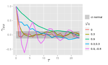
The autocorrelation function of an AR(p) process can be expressed as^{[citation needed]}

ρ(τ)=∑k=1pakyk−|τ|,{displaystyle rho (tau )=sum _{k=1}^{p}a_{k}y_{k}^{-|tau |},}

where yk{displaystyle y_{k}} are the roots of the polynomial

ϕ(B)=1−∑k=1pφkBk{displaystyle phi (B)=1-sum _{k=1}^{p}varphi _{k}B^{k}}

where B is the backshift operator, where ϕ(⋅){displaystyle phi (cdot )} is the function defining the autoregression, and where φk{displaystyle varphi _{k}} are the coefficients in the autoregression.

The autocorrelation function of an AR(p) process is a sum of decaying exponentials.

• Each real root contributes a component to the autocorrelation function that decays exponentially.


• Similarly, each pair of complex conjugate roots contributes an exponentially damped oscillation.

Graphs of AR(p) processes

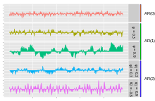
AR(0); AR(1) with AR parameter 0.3; AR(1) with AR parameter 0.9; AR(2) with AR parameters 0.3 and 0.3; and AR(2) with AR parameters 0.9 and −0.8

The simplest AR process is AR(0), which has no dependence between the terms. Only the error/innovation/noise term contributes to the output of the process, so in the figure, AR(0) corresponds to white noise.

For an AR(1) process with a positive φ{displaystyle varphi }, only the previous term in the process and the noise term contribute to the output. If φ{displaystyle varphi } is close to 0, then the process still looks like white noise, but as φ{displaystyle varphi } approaches 1, the output gets a larger contribution from the previous term relative to the noise. This results in a "smoothing" or integration of the output, similar to a low pass filter.

For an AR(2) process, the previous two terms and the noise term contribute to the output. If both φ1{displaystyle varphi _{1}} and φ2{displaystyle varphi _{2}} are positive, the output will resemble a low pass filter, with the high frequency part of the noise decreased. If φ1{displaystyle varphi _{1}} is positive while φ2{displaystyle varphi _{2}} is negative, then the process favors changes in sign between terms of the process. The output oscillates. This can be likened to edge detection or detection of change in direction.

Example: An AR(1) process

An AR(1) process is given by:

Xt=c+φXt−1+εt{displaystyle X_{t}=c+varphi X_{t-1}+varepsilon _{t},}

where εt{displaystyle varepsilon _{t}} is a white noise process with zero mean and constant variance σε2{displaystyle sigma _{varepsilon }^{2}}.
(Note: The subscript on φ1{displaystyle varphi _{1}} has been dropped.) The process is wide-sense stationary if |φ|<1{displaystyle |varphi |<1} since it is obtained as the output of a stable filter whose input is white noise. (If φ=1{displaystyle varphi =1} then Xt{displaystyle X_{t}} has infinite variance, and is therefore not wide sense stationary.) Assuming |φ|<1{displaystyle |varphi |<1}, the mean E⁡(Xt){displaystyle operatorname {E} (X_{t})} is identical for all values of t by the very definition of wide sense stationarity. If the mean is denoted by μ{displaystyle mu }, it follows from

E⁡(Xt)=E⁡(c)+φE⁡(Xt−1)+E⁡(εt),{displaystyle operatorname {E} (X_{t})=operatorname {E} (c)+varphi operatorname {E} (X_{t-1})+operatorname {E} (varepsilon _{t}),}

that

μ=c+φμ+0,{displaystyle mu =c+varphi mu +0,}

and hence

μ=c1−φ.{displaystyle mu ={frac {c}{1-varphi }}.}

In particular, if c=0{displaystyle c=0}, then the mean is 0.

The variance is

var(Xt)=E⁡(Xt2)−μ2=σε21−φ2,{displaystyle {textrm {var}}(X_{t})=operatorname {E} (X_{t}^{2})-mu ^{2}={frac {sigma _{varepsilon }^{2}}{1-varphi ^{2}}},}

where σε{displaystyle sigma _{varepsilon }} is the standard deviation of εt{displaystyle varepsilon _{t}}. This can be shown by noting that

var(Xt)=φ2var(Xt−1)+σε2,{displaystyle {textrm {var}}(X_{t})=varphi ^{2}{textrm {var}}(X_{t-1})+sigma _{varepsilon }^{2},}

and then by noticing that the quantity above is a stable fixed point of this relation.

The autocovariance is given by

Bn=E⁡(Xt+nXt)−μ2=σε21−φ2φ|n|.{displaystyle B_{n}=operatorname {E} (X_{t+n}X_{t})-mu ^{2}={frac {sigma _{varepsilon }^{2}}{1-varphi ^{2}}},,varphi ^{|n|}.}

It can be seen that the autocovariance function decays with a decay time (also called time constant) of τ=−1/ln⁡(φ){displaystyle tau =-1/ln(varphi )} [to see this, write Bn=Kφ|n|{displaystyle B_{n}=Kvarphi ^{|n|}} where K{displaystyle K} is independent of n{displaystyle n}. Then note that φ|n|=e|n|ln⁡φ{displaystyle varphi ^{|n|}=e^{|n|ln varphi }} and match this to the exponential decay law e−n/τ{displaystyle e^{-n/tau }}].

The spectral density function is the Fourier transform of the autocovariance function. In discrete terms this will be the discrete-time Fourier transform:

Φ(ω)=12π∑n=−∞∞Bne−iωn=12π(σε21+φ2−2φcos⁡(ω)).{displaystyle Phi (omega )={frac {1}{sqrt {2pi }}},sum _{n=-infty }^{infty }B_{n}e^{-iomega n}={frac {1}{sqrt {2pi }}},left({frac {sigma _{varepsilon }^{2}}{1+varphi ^{2}-2varphi cos(omega )}}right).}

This expression is periodic due to the discrete nature of the Xj{displaystyle X_{j}}, which is manifested as the cosine term in the denominator. If we assume that the sampling time (Δt=1{displaystyle Delta t=1}) is much smaller than the decay time (τ{displaystyle tau }), then we can use a continuum approximation to Bn{displaystyle B_{n}}:

B(t)≈σε21−φ2φ|t|{displaystyle B(t)approx {frac {sigma _{varepsilon }^{2}}{1-varphi ^{2}}},,varphi ^{|t|}}

which yields a Lorentzian profile for the spectral density:

Φ(ω)=12πσε21−φ2γπ(γ2+ω2){displaystyle Phi (omega )={frac {1}{sqrt {2pi }}},{frac {sigma _{varepsilon }^{2}}{1-varphi ^{2}}},{frac {gamma }{pi (gamma ^{2}+omega ^{2})}}}

where γ=1/τ{displaystyle gamma =1/tau } is the angular frequency associated with the decay time τ{displaystyle tau }.

An alternative expression for Xt{displaystyle X_{t}} can be derived by first substituting c+φXt−2+εt−1{displaystyle c+varphi X_{t-2}+varepsilon _{t-1}} for Xt−1{displaystyle X_{t-1}} in the defining equation. Continuing this process N times yields

Xt=c∑k=0N−1φk+φNXt−N+∑k=0N−1φkεt−k.{displaystyle X_{t}=csum _{k=0}^{N-1}varphi ^{k}+varphi ^{N}X_{t-N}+sum _{k=0}^{N-1}varphi ^{k}varepsilon _{t-k}.}

For N approaching infinity, φN{displaystyle varphi ^{N}} will approach zero and:

Xt=c1−φ+∑k=0∞φkεt−k.{displaystyle X_{t}={frac {c}{1-varphi }}+sum _{k=0}^{infty }varphi ^{k}varepsilon _{t-k}.}

It is seen that Xt{displaystyle X_{t}} is white noise convolved with the φk{displaystyle varphi ^{k}} kernel plus the constant mean. If the white noise εt{displaystyle varepsilon _{t}} is a Gaussian process then Xt{displaystyle X_{t}} is also a Gaussian process. In other cases, the central limit theorem indicates that Xt{displaystyle X_{t}} will be approximately normally distributed when φ{displaystyle varphi } is close to one.

Explicit mean/difference form of AR(1) process

The AR(1) model is the discrete time analogy of the continuous Ornstein-Uhlenbeck process. It is therefore sometimes useful to understand the properties of the AR(1) model cast in an equivalent form. In this form, the AR(1) model, with process parameter θ{displaystyle theta } is given by:

Xt+1=Xt+(1−θ)(μ−Xt)+ϵt+1{displaystyle X_{t+1}=X_{t}+(1-theta )(mu -X_{t})+epsilon _{t+1},}, where |θ|<1{displaystyle |theta |<1,} and μ{displaystyle mu } is the model mean.

By putting this in the form Xt+1=c+ϕXt{displaystyle X_{t+1}=c+phi X_{t},}, and then expanding the series for Xt+n{displaystyle X_{t+n}}, one can show that:

E⁡(Xt+n|Xt)=μ[1−θn]+Xtθn{displaystyle operatorname {E} (X_{t+n}|X_{t})=mu left[1-theta ^{n}right]+X_{t}theta ^{n}}, and

Var⁡(Xt+n|Xt)=σ21−θ2n1−θ2{displaystyle operatorname {Var} (X_{t+n}|X_{t})=sigma ^{2}{frac {1-theta ^{2n}}{1-theta ^{2}}}}.

Choosing the maximum lag

The partial autocorrelation of an AR(p) process is zero at lag p + 1 and greater, so the appropriate maximum lag is the one beyond which the partial autocorrelations are all zero.

Calculation of the AR parameters

There are many ways to estimate the coefficients, such as the ordinary least squares procedure or method of moments (through Yule–Walker equations).

The AR(p) model is given by the equation

Xt=∑i=1pφiXt−i+εt.{displaystyle X_{t}=sum _{i=1}^{p}varphi _{i}X_{t-i}+varepsilon _{t}.,}

It is based on parameters φi{displaystyle varphi _{i}} where i = 1, ..., p. There is a direct correspondence between these parameters and the covariance function of the process, and this correspondence can be inverted to determine the parameters from the autocorrelation function (which is itself obtained from the covariances). This is done using the Yule–Walker equations.

Yule–Walker equations

The Yule–Walker equations, named for Udny Yule and Gilbert Walker,^[1][2] are the following set of equations.^[3]

γm=∑k=1pφkγm−k+σε2δm,0,{displaystyle gamma _{m}=sum _{k=1}^{p}varphi _{k}gamma _{m-k}+sigma _{varepsilon }^{2}delta _{m,0},}

where m = 0, ..., p, yielding p + 1 equations. Here γm{displaystyle gamma _{m}} is the autocovariance function of X_t, σε{displaystyle sigma _{varepsilon }} is the standard deviation of the input noise process, and δm,0{displaystyle delta _{m,0}} is the Kronecker delta function.

Because the last part of an individual equation is non-zero only if m = 0, the set of equations can be solved by representing the equations for m > 0 in matrix form, thus getting the equation

[γ1γ2γ3⋮γp]=[γ0γ−1γ−2…γ1γ0γ−1…γ2γ1γ0…⋮⋮⋮⋱γp−1γp−2γp−3…][φ1φ2φ3⋮φp]{displaystyle {begin{bmatrix}gamma _{1}\gamma _{2}\gamma _{3}\vdots \gamma _{p}\end{bmatrix}}={begin{bmatrix}gamma _{0}&gamma _{-1}&gamma _{-2}&dots \gamma _{1}&gamma _{0}&gamma _{-1}&dots \gamma _{2}&gamma _{1}&gamma _{0}&dots \vdots &vdots &vdots &ddots \gamma _{p-1}&gamma _{p-2}&gamma _{p-3}&dots \end{bmatrix}}{begin{bmatrix}varphi _{1}\varphi _{2}\varphi _{3}\vdots \varphi _{p}\end{bmatrix}}}

which can be solved for all {φm;m=1,2,⋯,p}.{displaystyle {varphi _{m};m=1,2,cdots ,p}.} The remaining equation for m = 0 is

γ0=∑k=1pφkγ−k+σε2,{displaystyle gamma _{0}=sum _{k=1}^{p}varphi _{k}gamma _{-k}+sigma _{varepsilon }^{2},}

which, once {φm;m=1,2,⋯,p}{displaystyle {varphi _{m};m=1,2,cdots ,p}} are known, can be solved for σε2.{displaystyle sigma _{varepsilon }^{2}.}

An alternative formulation is in terms of the autocorrelation function. The AR parameters are determined by the first p+1 elements ρ(τ){displaystyle rho (tau )} of the autocorrelation function. The full autocorrelation function can then be derived by recursively calculating
^[4]

ρ(τ)=∑k=1pφkρ(k−τ){displaystyle rho (tau )=sum _{k=1}^{p}varphi _{k}rho (k-tau )}

Examples for some Low-order AR(p) processes

• p=1
  
  
  
  • γ1=φ1γ0{displaystyle gamma _{1}=varphi _{1}gamma _{0}}
  
  
  • Hence ρ1=γ1/γ0=φ1{displaystyle rho _{1}=gamma _{1}/gamma _{0}=varphi _{1}}
    
  
  
  
  


• p=2
  
  • The Yule–Walker equations for an AR(2) process are
    

    
    

    γ1=φ1γ0+φ2γ−1{displaystyle gamma _{1}=varphi _{1}gamma _{0}+varphi _{2}gamma _{-1}}

    
    

    γ2=φ1γ1+φ2γ0{displaystyle gamma _{2}=varphi _{1}gamma _{1}+varphi _{2}gamma _{0}}

    
    

    
    
    
    
    • Remember that γ−k=γk{displaystyle gamma _{-k}=gamma _{k}}
      
    
    
    • Using the first equation yields ρ1=γ1/γ0=φ11−φ2{displaystyle rho _{1}=gamma _{1}/gamma _{0}={frac {varphi _{1}}{1-varphi _{2}}}}
      
    
    
    • Using the recursion formula yields ρ2=γ2/γ0=φ12−φ22+φ21−φ2{displaystyle rho _{2}=gamma _{2}/gamma _{0}={frac {varphi _{1}^{2}-varphi _{2}^{2}+varphi _{2}}{1-varphi _{2}}}}
      
    
    
    
    
  
  

Estimation of AR parameters

The above equations (the Yule–Walker equations) provide several routes to estimating the parameters of an AR(p) model, by replacing the theoretical covariances with estimated values.^{[citation needed]} Some of these variants can be described as follows:

• Estimation of autocovariances or autocorrelations. Here each of these terms is estimated separately, using conventional estimates. There are different ways of doing this and the choice between these affects the properties of the estimation scheme. For example, negative estimates of the variance can be produced by some choices.


• Formulation as a least squares regression problem in which an ordinary least squares prediction problem is constructed, basing prediction of values of X_t on the p previous values of the same series. This can be thought of as a forward-prediction scheme. The normal equations for this problem can be seen to correspond to an approximation of the matrix form of the Yule–Walker equations in which each appearance of an autocovariance of the same lag is replaced by a slightly different estimate.


• Formulation as an extended form of ordinary least squares prediction problem. Here two sets of prediction equations are combined into a single estimation scheme and a single set of normal equations. One set is the set of forward-prediction equations and the other is a corresponding set of backward prediction equations, relating to the backward representation of the AR model:

Xt=c+∑i=1pφiXt−i+εt∗.{displaystyle X_{t}=c+sum _{i=1}^{p}varphi _{i}X_{t-i}+varepsilon _{t}^{*},.}

Here predicted of values of X_t would be based on the p future values of the same series. This way of estimating the AR parameters is due to Burg,^[5] and is called the Burg method:^[6] Burg and later authors called these particular estimates "maximum entropy estimates",^[7] but the reasoning behind this applies to the use of any set of estimated AR parameters. Compared to the estimation scheme using only the forward prediction equations, different estimates of the autocovariances are produced, and the estimates have different stability properties. Burg estimates are particularly associated with maximum entropy spectral estimation.^[8]

Other possible approaches to estimation include maximum likelihood estimation. Two distinct variants of maximum likelihood are available: in one (broadly equivalent to the forward prediction least squares scheme) the likelihood function considered is that corresponding to the conditional distribution of later values in the series given the initial p values in the series; in the second, the likelihood function considered is that corresponding to the unconditional joint distribution of all the values in the observed series. Substantial differences in the results of these approaches can occur if the observed series is short, or if the process is close to non-stationarity.

Spectrum

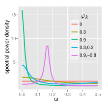
The power spectral density of an AR(p) process with noise variance Var(Zt)=σZ2{displaystyle mathrm {Var} (Z_{t})=sigma _{Z}^{2}} is^[4]

S(f)=σZ2|1−∑k=1pφke−i2πfk|2.{displaystyle S(f)={frac {sigma _{Z}^{2}}{|1-sum _{k=1}^{p}varphi _{k}e^{-i2pi fk}|^{2}}}.}

AR(0)

For white noise (AR(0))

S(f)=σZ2.{displaystyle S(f)=sigma _{Z}^{2}.}

AR(1)

For AR(1)

S(f)=σZ2|1−φ1e−2πif|2=σZ21+φ12−2φ1cos⁡2πf{displaystyle S(f)={frac {sigma _{Z}^{2}}{|1-varphi _{1}e^{-2pi if}|^{2}}}={frac {sigma _{Z}^{2}}{1+varphi _{1}^{2}-2varphi _{1}cos 2pi f}}}

• If φ1>0{displaystyle varphi _{1}>0} there is a single spectral peak at f=0, often referred to as red noise. As φ1{displaystyle varphi _{1}} becomes nearer 1, there is stronger power at low frequencies, i.e. larger time lags. This is then a low-pass filter, when applied to full spectrum light, everything except for the red light will be filtered.


• If φ1<0{displaystyle varphi _{1}<0} there is a minimum at f=0, often referred to as blue noise. This similarly acts as a high-pass filter, everything except for blue light will be filtered.

AR(2)

AR(2) processes can be split into three groups depending on the characteristics of their roots:

z1,z2=12(φ1±φ12+4φ2){displaystyle z_{1},z_{2}={frac {1}{2}}left(varphi _{1}pm {sqrt {varphi _{1}^{2}+4varphi _{2}}}right)}

• When φ12+4φ2<0{displaystyle varphi _{1}^{2}+4varphi _{2}<0}, the process has a pair of complex-conjugate roots, creating a mid-frequency peak at:

f∗=12πcos−1⁡(φ1(φ2−1)4φ2){displaystyle f^{*}={frac {1}{2pi }}cos ^{-1}left({frac {varphi _{1}(varphi _{2}-1)}{4varphi _{2}}}right)}

Otherwise the process has real roots, and:

• When φ1>0{displaystyle varphi _{1}>0} it acts as a low-pass filter on the white noise with a spectral peak at f=0{displaystyle f=0}
  


• When φ1<0{displaystyle varphi _{1}<0} it acts as a high-pass filter on the white noise with a spectral peak at f=1/2{displaystyle f=1/2}.

The process is non-stationary when the roots are outside the unit circle.
The process is stable when the roots are within the unit circle, or equivalently when the coefficients are in the triangle −1≤φ2≤1−|φ1|{displaystyle -1leq varphi _{2}leq 1-|varphi _{1}|}.

The full PSD function can be expressed in real form as:

S(f)=σZ21+φ12+φ22−2φ1(1−φ2)cos⁡(2πf)−2φ2cos⁡(4πf){displaystyle S(f)={frac {sigma _{Z}^{2}}{1+varphi _{1}^{2}+varphi _{2}^{2}-2varphi _{1}(1-varphi _{2})cos(2pi f)-2varphi _{2}cos(4pi f)}}}

Implementations in statistics packages

• 
  R, the stats package includes an ar function.^[9]
  


• 
  MATLAB's Econometrics Toolbox ^[10] and System Identification Toolbox ^[11] includes autoregressive models ^[12]
  


• 
  Matlab and Octave: the TSA toolbox contains several estimation functions for uni-variate, multivariate and adaptive autoregressive models.^[13]
  


• PyMC3: the Bayesian statistics and probabilistic programming framework supports autoregressive modes with p lags.


• 
  bayesloop supports parameter inference and model selection for the AR-1 process with time-varying parameters.^[14]
  

Impulse response

The impulse response of a system is the change in an evolving variable in response to a change in the value of a shock term k periods earlier, as a function of k. Since the AR model is a special case of the vector autoregressive model, the computation of the impulse response in vector autoregression#impulse response applies here.

n-step-ahead forecasting

Once the parameters of the autoregression

Xt=c+∑i=1pφiXt−i+εt{displaystyle X_{t}=c+sum _{i=1}^{p}varphi _{i}X_{t-i}+varepsilon _{t},}

have been estimated, the autoregression can be used to forecast an arbitrary number of periods into the future. First use t to refer to the first period for which data is not yet available; substitute the known preceding values X_t-i for i=1, ..., p into the autoregressive equation while setting the error term εt{displaystyle varepsilon _{t}} equal to zero (because we forecast X_t to equal its expected value, and the expected value of the unobserved error term is zero). The output of the autoregressive equation is the forecast for the first unobserved period. Next, use t to refer to the next period for which data is not yet available; again the autoregressive equation is used to make the forecast, with one difference: the value of X one period prior to the one now being forecast is not known, so its expected value—the predicted value arising from the previous forecasting step—is used instead. Then for future periods the same procedure is used, each time using one more forecast value on the right side of the predictive equation until, after p predictions, all p right-side values are predicted values from preceding steps.

There are four sources of uncertainty regarding predictions obtained in this manner: (1) uncertainty as to whether the autoregressive model is the correct model; (2) uncertainty about the accuracy of the forecasted values that are used as lagged values in the right side of the autoregressive equation; (3) uncertainty about the true values of the autoregressive coefficients; and (4) uncertainty about the value of the error term εt{displaystyle varepsilon _{t},} for the period being predicted. Each of the last three can be quantified and combined to give a confidence interval for the n-step-ahead predictions; the confidence interval will become wider as n increases because of the use of an increasing number of estimated values for the right-side variables.

Evaluating the quality of forecasts

The predictive performance of the autoregressive model can be assessed as soon as estimation has been done if cross-validation is used. In this approach, some of the initially available data was used for parameter estimation purposes, and some (from available observations later in the data set) was held back for out-of-sample testing. Alternatively, after some time has passed after the parameter estimation was conducted, more data will have become available and predictive performance can be evaluated then using the new data.

In either case, there are two aspects of predictive performance that can be evaluated: one-step-ahead and n-step-ahead performance. For one-step-ahead performance, the estimated parameters are used in the autoregressive equation along with observed values of X for all periods prior to the one being predicted, and the output of the equation is the one-step-ahead forecast; this procedure is used to obtain forecasts for each of the out-of-sample observations. To evaluate the quality of n-step-ahead forecasts, the forecasting procedure in the previous section is employed to obtain the predictions.

Given a set of predicted values and a corresponding set of actual values for X for various time periods, a common evaluation technique is to use the mean squared prediction error; other measures are also available (see forecasting#forecasting accuracy).

The question of how to interpret the measured forecasting accuracy arises—for example, what is a "high" (bad) or a "low" (good) value for the mean squared prediction error? There are two possible points of comparison. First, the forecasting accuracy of an alternative model, estimated under different modeling assumptions or different estimation techniques, can be used for comparison purposes. Second, the out-of-sample accuracy measure can be compared to the same measure computed for the in-sample data points (that were used for parameter estimation) for which enough prior data values are available (that is, dropping the first p data points, for which p prior data points are not available). Since the model was estimated specifically to fit the in-sample points as well as possible, it will usually be the case that the out-of-sample predictive performance will be poorer than the in-sample predictive performance. But if the predictive quality deteriorates out-of-sample by "not very much" (which is not precisely definable), then the forecaster may be satisfied with the performance.

See also

• Moving average model


• Linear difference equation


• Predictive analytics


• Linear predictive coding


• Resonance


• Levinson recursion

Notes

References

• 
  Mills, Terence C. (1990). Time Series Techniques for Economists. Cambridge University Press.
  


• 
  Percival, Donald B.; Walden, Andrew T. (1993). Spectral Analysis for Physical Applications. Cambridge University Press.
  


• 
  Pandit, Sudhakar M.; Wu, Shien-Ming (1983). Time Series and System Analysis with Applications. John Wiley & Sons.
  

External links

• 
  AutoRegression Analysis (AR) by Paul Bourke


• 
  Econometrics lecture (topic: Autoregressive models) on YouTube by Mark Thoma