Wsrtjtyk

Quantum mechanical operator related to rotational symmetry

In quantum mechanics, the angular momentum operator is one of several related operators analogous to classical angular momentum. The angular momentum operator plays a central role in the theory of atomic physics and other quantum problems involving rotational symmetry. In both classical and quantum mechanical systems, angular momentum (together with linear momentum and energy) is one of the three fundamental properties of motion.^[1]

There are several angular momentum operators: total angular momentum (usually denoted J), orbital angular momentum (usually denoted L), and spin angular momentum (spin for short, usually denoted S). The term angular momentum operator can (confusingly) refer to either the total or the orbital angular momentum. Total angular momentum is always conserved, see Noether's theorem.

Overview

"Vector cones" of total angular momentum J (purple), orbital L (blue), and spin S (green). The cones arise due to quantum uncertainty between measuring angular momentum components (see below).

In quantum mechanics, angular momentum can refer to one of three different, but related things.

Orbital angular momentum

The classical definition of angular momentum is $mathbf{L} = mathbf{r} times mathbf{p}$ . The quantum-mechanical counterparts of these objects share the same relationship:

mathbf{L} = mathbf{r} times mathbf{p}

where r is the quantum position operator, p is the quantum momentum operator, × is cross product, and L is the orbital angular momentum operator. L (just like p and r) is a vector operator (a vector whose components are operators), i.e. ${displaystyle mathbf {L} =left(L_{x},L_{y},L_{z}right)}$ where L_x, L_y, L_z are three different quantum-mechanical operators.

In the special case of a single particle with no electric charge and no spin, the orbital angular momentum operator can be written in the position basis as:

{displaystyle mathbf {L} =-ihbar (mathbf {r} times nabla )}

where ∇ is the vector differential operator, del.

Spin angular momentum

There is another type of angular momentum, called spin angular momentum (more often shortened to spin), represented by the spin operator S. Spin is often depicted as a particle literally spinning around an axis, but this is only a metaphor: spin is an intrinsic property of a particle, unrelated to any sort of motion in space. All elementary particles have a characteristic spin, which is usually nonzero. For example, electrons always have "spin 1/2" while photons always have "spin 1" (details below).

Total angular momentum

Finally, there is total angular momentum J, which combines both the spin and orbital angular momentum of a particle or system:

{displaystyle mathbf {J} =mathbf {L} +mathbf {S} .}

Conservation of angular momentum states that J for a closed system, or J for the whole universe, is conserved. However, L and S are not generally conserved. For example, the spin–orbit interaction allows angular momentum to transfer back and forth between L and S, with the total J remaining constant.

Commutation relations

Commutation relations between components

The orbital angular momentum operator is a vector operator, meaning it can be written in terms of its vector components ${displaystyle mathbf {L} =left(L_{x},L_{y},L_{z}right)}$ . The components have the following commutation relations with each other:^[2]

{displaystyle left[L_{x},L_{y}right]=ihbar L_{z},;;left[L_{y},L_{z}right]=ihbar L_{x},;;left[L_{z},L_{x}right]=ihbar L_{y},}

where [ , ] denotes the commutator

{displaystyle [X,Y]equiv XY-YX.}

This can be written generally as

{displaystyle left[L_{l},L_{m}right]=ihbar sum _{n=1}^{3}varepsilon _{lmn}L_{n}}

,

where l, m, n are the component indices (1 for x, 2 for y, 3 for z), and ε_lmn denotes the Levi-Civita symbol.

A compact expression as one vector equation is also possible:^[3]

{displaystyle mathbf {L} times mathbf {L} =ihbar mathbf {L} }

The commutation relations can be proved as a direct consequence of the canonical commutation relations $[x_{l},p_{m}]=ihbar delta _{lm}$ , where δ_lm is the Kronecker delta.

There is an analogous relationship in classical physics:^[4]

{displaystyle left{L_{i},L_{j}right}=varepsilon _{ijk}L_{k}}

where L_n is a component of the classical angular momentum operator, and ${,}$ is the Poisson bracket.

The same commutation relations apply for the other angular momentum operators (spin and total angular momentum):^[5]

{displaystyle left[S_{l},S_{m}right]=ihbar sum _{n=1}^{3}varepsilon _{lmn}S_{n},quad left[J_{l},J_{m}right]=ihbar sum _{n=1}^{3}varepsilon _{lmn}J_{n}}

.

These can be assumed to hold in analogy with L. Alternatively, they can be derived as discussed below.

These commutation relations mean that L has the mathematical structure of a Lie algebra, and the ε_lmn are its structure constants. In this case, the Lie algebra is SU(2) or SO(3) in physics notation ( ${displaystyle operatorname {su} (2)}$ or ${displaystyle operatorname {so} (3)}$ respectively in mathematics notation), i.e. Lie algebra associated with rotations in three dimensions. The same is true of J and S. The reason is discussed below. These commutation relations are relevant for measurement and uncertainty, as discussed further below.

Commutation relations involving vector magnitude

Like any vector, a magnitude can be defined for the orbital angular momentum operator,

L^{2}equiv L_{x}^{2}+L_{y}^{2}+L_{z}^{2}

.

L² is another quantum operator. It commutes with the components of L,

{displaystyle left[L^{2},L_{x}right]=left[L^{2},L_{y}right]=left[L^{2},L_{z}right]=0~.,}

One way to prove that these operators commute is to start from the [L_ℓ, L_m] commutation relations in the previous section:

Click [show] on the right to see a proof of [L², L_x] = 0, starting from the [L_ℓ, L_m] commutation relations^[6]
${displaystyle {begin{aligned}left[L^{2},L_{x}right]&=left[L_{x}^{2},L_{x}right]+left[L_{y}^{2},L_{x}right]+left[L_{z}^{2},L_{x}right]\&=L_{y}left[L_{y},L_{x}right]+left[L_{y},L_{x}right]L_{y}+L_{z}left[L_{z},L_{x}right]+left[L_{z},L_{x}right]L_{z}\&=L_{y}left(-ihbar L_{z}right)+left(-ihbar L_{z}right)L_{y}+L_{z}left(ihbar L_{y}right)+left(ihbar L_{y}right)L_{z}\&=0end{aligned}}}$

Mathematically, L² is a Casimir invariant of the Lie algebra SO(3) spanned by L.

As above, there is an analogous relationship in classical physics:

{displaystyle left{L^{2},L_{x}right}=left{L^{2},L_{y}right}=left{L^{2},L_{z}right}=0}

where L_i is a component of the classical angular momentum operator, and ${,}$ is the Poisson bracket.^[7]

Returning to the quantum case, the same commutation relations apply to the other angular momentum operators (spin and total angular momentum), as well,

{displaystyle {begin{aligned}leftlbrack S^{2},S_{i}rightrbrack &=0,\leftlbrack J^{2},J_{i}rightrbrack &=0.end{aligned}}}

Uncertainty principle

In general, in quantum mechanics, when two observable operators do not commute, they are called complementary observables. Two complementary observables cannot be measured simultaneously; instead they satisfy an uncertainty principle. The more accurately one observable is known, the less accurately the other one can be known. Just as there is an uncertainty principle relating position and momentum, there are uncertainty principles for angular momentum.

The Robertson–Schrödinger relation gives the following uncertainty principle:

sigma _{L_{x}}sigma _{L_{y}}geq {frac {hbar }{2}}left|langle L_{z}rangle right|.

where $sigma _{X}$ is the standard deviation in the measured values of X and $langle Xrangle$ denotes the expectation value of X. This inequality is also true if x, y, z are rearranged, or if L is replaced by J or S.

Therefore, two orthogonal components of angular momentum (for example L_x and L_y) are complementary and cannot be simultaneously known or measured, except in special cases such as ${displaystyle L_{x}=L_{y}=L_{z}=0}$ .

It is, however, possible to simultaneously measure or specify L² and any one component of L; for example, L² and L_z. This is often useful, and the values are characterized by the azimuthal quantum number (l) and the magnetic quantum number (m). In this case the quantum state of the system is a simultaneous eigenstate of the operators L² and L_z, but not of L_x or L_y. The eigenvalues are related to l and m, as shown in the table below.

Quantization

In quantum mechanics, angular momentum is quantized – that is, it cannot vary continuously, but only in "quantum leaps" between certain allowed values. For any system, the following restrictions on measurement results apply, where $hbar$ is reduced Planck constant:

If you measure...	...the result can be...	Notes
$L_{z}$	$(hbar m)$ , where ${displaystyle min {ldots ,-2,-1,0,1,2,ldots }}$	m is sometimes called magnetic quantum number. This same quantization rule holds for any component of L; e.g., L_x or L_y. This rule is sometimes called spatial quantization.^[8]
$S_{z}$ or $J_{z}$	$(hbar m)$ , where ${displaystyle min {ldots ,-1,-0.5,0,0.5,1,1.5,ldots }}$	For S_z, m is sometimes called spin projection quantum number. For J_z, m is sometimes called total angular momentum projection quantum number. This same quantization rule holds for any component of S or J; e.g., S_x or J_y.
$L^{2}$	${displaystyle left(hbar ^{2}ell (ell +1)right)}$ , where ${displaystyle ell in {0,1,2,ldots }}$	L² is defined by $L^{2}equiv L_{x}^{2}+L_{y}^{2}+L_{z}^{2}$ . $ell$ is sometimes called azimuthal quantum number or orbital quantum number.
$S^{2}$	${displaystyle left(hbar ^{2}s(s+1)right)}$ , where ${displaystyle sin {0,0.5,1,1.5,ldots }}$	s is called spin quantum number or just spin. For example, a spin-½ particle is a particle where s = ½.
$J^{2}$	${displaystyle left(hbar ^{2}j(j+1)right)}$ , where ${displaystyle jin {0,0.5,1,1.5,ldots }}$	j is sometimes called total angular momentum quantum number.
$L^{2}$ and $L_{z}$ simultaneously	${displaystyle left(hbar ^{2}ell (ell +1)right)}$ for $L^{2}$ , and ${displaystyle left(hbar m_{ell }right)}$ for $L_{z}$ where ${displaystyle ell in {0,1,2,ldots }}$ and ${displaystyle m_{ell }in {-ell ,(-ell +1),ldots ,(ell -1),ell }}$	(See above for terminology.)
$S^{2}$ and $S_{z}$ simultaneously	${displaystyle left(hbar ^{2}s(s+1)right)}$ for $S^{2}$ , and ${displaystyle left(hbar m_{s}right)}$ for $S_{z}$ where ${displaystyle sin {0,0.5,1,1.5,ldots }}$ and ${displaystyle m_{s}in {-s,(-s+1),ldots ,(s-1),s}}$	(See above for terminology.)
$J^{2}$ and $J_{z}$ simultaneously	${displaystyle left(hbar ^{2}j(j+1)right)}$ for $J^{2}$ , and ${displaystyle left(hbar m_{j}right)}$ for $J_{z}$ where ${displaystyle jin {0,0.5,1,1.5,ldots }}$ and ${displaystyle m_{j}in {-j,(-j+1),ldots ,(j-1),j}}$	(See above for terminology.)

In this standing wave on a circular string, the circle is broken into exactly 8 wavelengths. A standing wave like this can have 0, 1, 2, or any integer number of wavelengths around the circle, but it cannot have a non-integer number of wavelengths like 8.3. In quantum mechanics, angular momentum is quantized for a similar reason.

Derivation using ladder operators

A common way to derive the quantization rules above is the method of ladder operators.^[9] The ladder operators are defined:

{begin{aligned}J_{+}&equiv J_{x}+iJ_{y},\J_{-}&equiv J_{x}-iJ_{y}end{aligned}}

Suppose a state $|psi rangle$ is a state in the simultaneous eigenbasis of $J^{2}$ and $J_{z}$ (i.e., a state with a single, definite value of $J^{2}$ and a single, definite value of $J_{z}$ ). Then using the commutation relations, one can prove that ${displaystyle J_{+}|psi rangle }$ and $J_{-}|psi rangle$ are also in the simultaneous eigenbasis, with the same value of $J^{2}$ , but where $J_{z}|psi rangle$ is increased or decreased by $hbar$ , respectively. (It is also possible that one or both of these result vectors is the zero vector.) (For a proof, see ladder operator#Angular momentum.)

By manipulating these ladder operators and using the commutation rules, it is possible to prove almost all of the quantization rules above.

Click [show] on the right to see more details in the ladder-operator proof of the quantization rules^[9]

Before starting the main proof, we will note a useful fact: That

{displaystyle J_{x}^{2},J_{y}^{2},J_{z}^{2}}

are positive-semidefinite operators, meaning that all their eigenvalues are nonnegative. That also implies that the same is true for their sums, including

J^{2}=J_{x}^{2}+J_{y}^{2}+J_{z}^{2}

and

{displaystyle left(J^{2}-J_{z}^{2}right)=left(J_{x}^{2}+J_{y}^{2}right)}

. The reason is that the square of any Hermitian operator is always positive semidefinite. (A Hermitian operator has real eigenvalues, so the squares of those eigenvalues are nonnegative.)

As above, assume that a state $|psi rangle$ is a state in the simultaneous eigenbasis of $J^{2}$ and $J_{z}$ . Its eigenvalue with respect to $J^{2}$ can be written in the form ${displaystyle hbar ^{2}j(j+1)}$ for some real number j > 0 (because as mentioned in the previous paragraph, $J^{2}$ has nonnegative eigenvalues), and its eigenvalue with respect to $J_{z}$ can be written $hbar m$ for some real number m. Instead of $|psi rangle$ we will use the more descriptive notation ${displaystyle |psi rangle =|j,mrangle }$ .

Next, consider the sequence ("ladder") of states

{displaystyle {ldots ;,;J_{-}J_{-}|j,mrangle ,;J_{-}|j,mrangle ,;|j,mrangle ,;J_{+}|j,mrangle ,;J_{+}J_{+}|j,mrangle ,;ldots }}

Some entries in this infinite sequence may be the zero vector (as we will see). However, as described above, all the nonzero entries have the same value of $J^{2}$ , and among the nonzero entries, each entry has a value of $J_{z}$ which is exactly $hbar$ more than the previous entry.

In this ladder, there can only be a finite number of nonzero entries, with infinite copies of the zero vector on the left and right. The reason is, as mentioned above, $(J^{2}-J_{z}^{2})$ is positive-semidefinite, so if any quantum state is an eigenvector of both $J^{2}$ and $J_{z}^{2}$ , the former eigenvalue is larger. The states in the ladder all have the same $J^{2}$ eigenvalue, but going very far to the left or the right, the $J_{z}^{2}$ eigenvalue gets larger and larger. The only possible resolution is, as mentioned, that there are only finitely many nonzero entries in the ladder.

Now, consider the last nonzero entry to the right of the ladder, $|j,m_{max}rangle$ . This state has the property that $J_{+}|j,m_{max}rangle =0$ . As proven in the ladder operator article,

{displaystyle J_{+}|j,mrangle =hbar {sqrt {j(j+1)-m(m+1)}}|j,m+1rangle }

If this is zero, then ${displaystyle j(j+1)=m_{text{max}}left(m_{text{max}}+1right)}$ , so ${displaystyle j=m}$ or $j=-m-1$ . However, because $J^{2}-J_{z}^{2}$ is positive-semidefinite, ${displaystyle hbar ^{2}j(j+1)geq (hbar m)^{2}}$ , which means that the only possibility is ${displaystyle m_{text{max}}=j}$ .

Similarly, consider the first nonzero entry on the left of the ladder, ${displaystyle |j,m_{text{min}}rangle }$ . This state has the property that ${displaystyle J_{-}left|j,m_{text{min}}rightrangle =0}$ . As proven in the ladder operator article,

{displaystyle J_{-}|j,mrangle =hbar {sqrt {j(j+1)-m(m-1)}}|j,m-1rangle }

As above, the only possibility is that ${displaystyle m_{text{min}}=-j}$

Since m changes by 1 on each step of the ladder, $(j-(-j))$ is an integer, so j is an integer or half-integer (0 or 0.5 or 1 or 1.5...).

Since S and L have the same commutation relations as J, the same ladder analysis works for them.

The ladder-operator analysis does not explain one aspect of the quantization rules above: the fact that L (unlike J and S) cannot have half-integer quantum numbers. This fact can be proven (at least in the special case of one particle) by writing down every possible eigenfunction of L² and L_z, (they are the spherical harmonics), and seeing explicitly that none of them have half-integer quantum numbers.^[10] An alternative derivation is below.

Visual interpretation

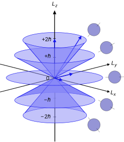
Illustration of the vector model of orbital angular momentum.

Since the angular momenta are quantum operators, they cannot be drawn as vectors like in classical mechanics. Nevertheless, it is common to depict them heuristically in this way. Depicted on the right is a set of states with quantum numbers $ell =2$ , and ${displaystyle m_{ell }=-2,-1,0,1,2}$ for the five cones from bottom to top. Since ${displaystyle |L|={sqrt {L^{2}}}=hbar {sqrt {6}}}$ , the vectors are all shown with length $hbar {sqrt {6}}$ . The rings represent the fact that $L_{z}$ is known with certainty, but $L_{x}$ and $L_{y}$ are unknown; therefore every classical vector with the appropriate length and z-component is drawn, forming a cone. The expected value of the angular momentum for a given ensemble of systems in the quantum state characterized by $ell$ and $m_{ell }$ could be somewhere on this cone while it cannot be defined for a single system (since the components of $L$ do not commute with each other).

Quantization in macroscopic systems

The quantization rules are technically true even for macroscopic systems, like the angular momentum L of a spinning tire. However they have no observable effect. For example, if $L_{z}/hbar$ is roughly 100000000, it makes essentially no difference whether the precise value is an integer like 100000000 or 100000001, or a non-integer like 100000000.2—the discrete steps are too small to notice.

Angular momentum as the generator of rotations

The most general and fundamental definition of angular momentum is as the generator of rotations.^[5] More specifically, let $R({hat {n}},phi )$ be a rotation operator, which rotates any quantum state about axis ${hat {n}}$ by angle $phi$ . As $phi rightarrow 0$ , the operator $R({hat {n}},phi )$ approaches the identity operator, because a rotation of 0° maps all states to themselves. Then the angular momentum operator $J_{hat {n}}$ about axis ${hat {n}}$ is defined as:^[5]

{displaystyle J_{hat {n}}equiv ihbar lim _{phi rightarrow 0}{frac {Rleft({hat {n}},phi right)-1}{phi }}=left.ihbar {frac {partial Rleft({hat {n}},phi right)}{partial phi }}right|_{phi =0}}

where 1 is the identity operator. Also notice that R is an additive morphism : ${displaystyle Rleft({hat {n}},phi _{1}+phi _{2}right)=Rleft({hat {n}},phi _{1}right)Rleft({hat {n}},phi _{2}right)}$ ; as a consequence^[5]

{displaystyle Rleft({hat {n}},phi right)=exp left(-{frac {iphi J_{hat {n}}}{hbar }}right)}

where exp is matrix exponential.

In simpler terms, the total angular momentum operator characterizes how a quantum system is changed when it is rotated. The relationship between angular momentum operators and rotation operators is the same as the relationship between Lie algebras and Lie groups in mathematics, as discussed further below.

The different types of rotation operators. The top box shows two particles, with spin states indicated schematically by the arrows.

The operator R, related to J, rotates the entire system.

The operator R_spatial, related to L, rotates the particle positions without altering their internal spin states.

The operator R_internal, related to S, rotates the particles' internal spin states without changing their positions.

Just as J is the generator for rotation operators, L and S are generators for modified partial rotation operators. The operator

{displaystyle R_{text{spatial}}left({hat {n}},phi right)=exp left(-{frac {iphi L_{hat {n}}}{hbar }}right),}

rotates the position (in space) of all particles and fields, without rotating the internal (spin) state of any particle. Likewise, the operator

{displaystyle R_{text{internal}}left({hat {n}},phi right)=exp left(-{frac {iphi S_{hat {n}}}{hbar }}right),}

rotates the internal (spin) state of all particles, without moving any particles or fields in space. The relation J = L + S comes from:

{displaystyle Rleft({hat {n}},phi right)=R_{text{internal}}left({hat {n}},phi right)R_{text{spatial}}left({hat {n}},phi right)}

i.e. if the positions are rotated, and then the internal states are rotated, then altogether the complete system has been rotated.

SU(2), SO(3), and 360° rotations

Although one might expect ${displaystyle Rleft({hat {n}},360^{circ }right)=1}$ (a rotation of 360° is the identity operator), this is not assumed in quantum mechanics, and it turns out it is often not true: When the total angular momentum quantum number is a half-integer (1/2, 3/2, etc.), ${displaystyle Rleft({hat {n}},360^{circ }right)=-1}$ , and when it is an integer, ${displaystyle Rleft({hat {n}},360^{circ }right)=+1}$ .^[5] Mathematically, the structure of rotations in the universe is not SO(3), the group of three-dimensional rotations in classical mechanics. Instead, it is SU(2), which is identical to SO(3) for small rotations, but where a 360° rotation is mathematically distinguished from a rotation of 0°. (A rotation of 720° is, however, the same as a rotation of 0°.)^[5]

On the other hand, ${displaystyle R_{text{spatial}}left({hat {n}},360^{circ }right)=+1}$ in all circumstances, because a 360° rotation of a spatial configuration is the same as no rotation at all. (This is different from a 360° rotation of the internal (spin) state of the particle, which might or might not be the same as no rotation at all.) In other words, the ${displaystyle R_{text{spatial}}}$ operators carry the structure of SO(3), while $R$ and ${displaystyle R_{text{internal}}}$ carry the structure of SU(2).

From the equation ${displaystyle +1=R_{text{spatial}}left({hat {z}},360^{circ }right)=exp left(-2pi iL_{z}/hbar right)}$ , one picks an eigenstate ${displaystyle L_{z}|psi rangle =mhbar |psi rangle }$ and draws

{displaystyle e^{-2pi im}=1}

which is to say that the orbital angular momentum quantum numbers can only be integers, not half-integers.

Connection to representation theory

Starting with a certain quantum state $|psi _{0}rangle$ , consider the set of states ${displaystyle Rleft({hat {n}},phi right)left|psi _{0}rightrangle }$ for all possible ${hat {n}}$ and $phi$ , i.e. the set of states that come about from rotating the starting state in every possible way. This is a vector space, and therefore the manner in which the rotation operators map one state onto another is a representation of the group of rotation operators.

When rotation operators act on quantum states, it forms a representation of the Lie group SU(2) (for R and R_internal), or SO(3) (for R_spatial).

From the relation between J and rotation operators,

When angular momentum operators act on quantum states, it forms a representation of the Lie algebra ${mathfrak {su}}(2)$ or ${mathfrak {so}}(3)$ .

(The Lie algebras of SU(2) and SO(3) are identical.)

The ladder operator derivation above is a method for classifying the representations of the Lie algebra SU(2).

Connection to commutation relations

Classical rotations do not commute with each other: For example, rotating 1° about the x-axis then 1° about the y-axis gives a slightly different overall rotation than rotating 1° about the y-axis then 1° about the x-axis. By carefully analyzing this noncommutativity, the commutation relations of the angular momentum operators can be derived.^[5]

(This same calculational procedure is one way to answer the mathematical question "What is the Lie algebra of the Lie groups SO(3) or SU(2)?")

Conservation of angular momentum

The Hamiltonian H represents the energy and dynamics of the system. In a spherically-symmetric situation, the Hamiltonian is invariant under rotations:

{displaystyle RHR^{-1}=H}

where R is a rotation operator. As a consequence, ${displaystyle [H,R]=0}$ , and then $[H,mathbf {J} ]=mathbf {0}$ due to the relationship between J and R. By the Ehrenfest theorem, it follows that J is conserved.

To summarize, if H is rotationally-invariant (spherically symmetric), then total angular momentum J is conserved. This is an example of Noether's theorem.

If H is just the Hamiltonian for one particle, the total angular momentum of that one particle is conserved when the particle is in a central potential (i.e., when the potential energy function depends only on ${displaystyle left|mathbf {r} right|}$ ). Alternatively, H may be the Hamiltonian of all particles and fields in the universe, and then H is always rotationally-invariant, as the fundamental laws of physics of the universe are the same regardless of orientation. This is the basis for saying conservation of angular momentum is a general principle of physics.

For a particle without spin, J = L, so orbital angular momentum is conserved in the same circumstances. When the spin is nonzero, the spin-orbit interaction allows angular momentum to transfer from L to S or back. Therefore, L is not, on its own, conserved.

Angular momentum coupling

Often, two or more sorts of angular momentum interact with each other, so that angular momentum can transfer from one to the other. For example, in spin-orbit coupling, angular momentum can transfer between L and S, but only the total J = L + S is conserved. In another example, in an atom with two electrons, each has its own angular momentum J₁ and J₂, but only the total J = J₁ + J₂ is conserved.

In these situations, it is often useful to know the relationship between, on the one hand, states where ${displaystyle left(J_{1}right)_{z},left(J_{1}right)^{2},left(J_{2}right)_{z},left(J_{2}right)^{2}}$ all have definite values, and on the other hand, states where ${displaystyle left(J_{1}right)^{2},left(J_{2}right)^{2},J^{2},J_{z}}$ all have definite values, as the latter four are usually conserved (constants of motion). The procedure to go back and forth between these bases is to use Clebsch–Gordan coefficients.

One important result in this field is that a relationship between the quantum numbers for ${displaystyle left(J_{1}right)^{2},left(J_{2}right)^{2},J^{2}}$ :

{displaystyle jin left{left|j_{1}-j_{2}right|,left(left|j_{1}-j_{2}right|+1right),ldots ,left(j_{1}+j_{2}right)right}}

.

For an atom or molecule with J = L + S, the term symbol gives the quantum numbers associated with the operators $L^{2},S^{2},J^{2}$ .

Orbital angular momentum in spherical coordinates

Angular momentum operators usually occur when solving a problem with spherical symmetry in spherical coordinates. The angular momentum in the spatial representation is^[11]

{displaystyle {begin{aligned}mathbf {L} &=ihbar left({frac {hat {boldsymbol {theta }}}{sin(theta )}}{frac {partial }{partial phi }}-{hat {boldsymbol {phi }}}{frac {partial }{partial theta }}right)\&=ihbar left({hat {mathbf {x} }}left(sin(phi ){frac {partial }{partial theta }}+cot(theta )cos(phi ){frac {partial }{partial phi }}right)+{hat {mathbf {y} }}left(-cos(phi ){frac {partial }{partial theta }}+cot(theta )sin(phi ){frac {partial }{partial phi }}right)-{hat {mathbf {z} }}{frac {partial }{partial phi }}right)\L_{+}&=hbar e^{iphi }left({frac {partial }{partial theta }}+icot(theta ){frac {partial }{partial phi }}right),\L_{-}&=hbar e^{-iphi }left(-{frac {partial }{partial theta }}+icot(theta ){frac {partial }{partial phi }}right),\L^{2}&=-hbar ^{2}left({frac {1}{sin(theta )}}{frac {partial }{partial theta }}left(sin(theta ){frac {partial }{partial theta }}right)+{frac {1}{sin ^{2}(theta )}}{frac {partial ^{2}}{partial phi ^{2}}}right),\L_{z}&=-ihbar {frac {partial }{partial phi }}.end{aligned}}}

In spherical coordinates the angular part of the Laplace operator can be expressed by the angular momentum. This leads to the relation

{displaystyle Delta ={frac {1}{r^{2}}}{frac {partial }{partial r}}left(r^{2},{frac {partial }{partial r}}right)-{frac {L^{2}}{hbar ^{2}r^{2}}}.}

When solving to find eigenstates of the operator $L^{2}$ , we obtain the following

{displaystyle {begin{aligned}L^{2}|l,mrangle &=hbar ^{2}l(l+1)|l,mrangle \L_{z}|l,mrangle &=hbar m|l,mrangle end{aligned}}}

where

{displaystyle leftlangle theta ,phi |l,mrightrangle =Y_{l,m}(theta ,phi )}

are the spherical harmonics.

References

^ Introductory Quantum Mechanics, Richard L. Liboff, 2nd Edition, .mw-parser-output cite.citation{font-style:inherit}.mw-parser-output .citation q{quotes:"""""""'""'"}.mw-parser-output .citation .cs1-lock-free a{background:url("//upload.wikimedia.org/wikipedia/commons/thumb/6/65/Lock-green.svg/9px-Lock-green.svg.png")no-repeat;background-position:right .1em center}.mw-parser-output .citation .cs1-lock-limited a,.mw-parser-output .citation .cs1-lock-registration a{background:url("//upload.wikimedia.org/wikipedia/commons/thumb/d/d6/Lock-gray-alt-2.svg/9px-Lock-gray-alt-2.svg.png")no-repeat;background-position:right .1em center}.mw-parser-output .citation .cs1-lock-subscription a{background:url("//upload.wikimedia.org/wikipedia/commons/thumb/a/aa/Lock-red-alt-2.svg/9px-Lock-red-alt-2.svg.png")no-repeat;background-position:right .1em center}.mw-parser-output .cs1-subscription,.mw-parser-output .cs1-registration{color:#555}.mw-parser-output .cs1-subscription span,.mw-parser-output .cs1-registration span{border-bottom:1px dotted;cursor:help}.mw-parser-output .cs1-ws-icon a{background:url("//upload.wikimedia.org/wikipedia/commons/thumb/4/4c/Wikisource-logo.svg/12px-Wikisource-logo.svg.png")no-repeat;background-position:right .1em center}.mw-parser-output code.cs1-code{color:inherit;background:inherit;border:inherit;padding:inherit}.mw-parser-output .cs1-hidden-error{display:none;font-size:100%}.mw-parser-output .cs1-visible-error{font-size:100%}.mw-parser-output .cs1-maint{display:none;color:#33aa33;margin-left:0.3em}.mw-parser-output .cs1-subscription,.mw-parser-output .cs1-registration,.mw-parser-output .cs1-format{font-size:95%}.mw-parser-output .cs1-kern-left,.mw-parser-output .cs1-kern-wl-left{padding-left:0.2em}.mw-parser-output .cs1-kern-right,.mw-parser-output .cs1-kern-wl-right{padding-right:0.2em}
ISBN 0-201-54715-5

^ Aruldhas, G. (2004-02-01). "formula (8.8)". Quantum Mechanics. p. 171. ISBN 978-81-203-1962-2.

^ Shankar, R. (1994). Principles of quantum mechanics (2nd ed.). New York: Kluwer Academic / Plenum. p. 319. ISBN 9780306447907.

^ H. Goldstein, C. P. Poole and J. Safko, Classical Mechanics, 3rd Edition, Addison-Wesley 2002, pp. 388 ﬀ.

^ ^a^b^c^d^e^f^g Littlejohn, Robert (2011). "Lecture notes on rotations in quantum mechanics" (PDF). Physics 221B Spring 2011. Retrieved 13 Jan 2012.

^
Griffiths, David J. (1995). Introduction to Quantum Mechanics. Prentice Hall. p. 146.

^ Goldstein et al, p. 410

^ Introduction to quantum mechanics: with applications to chemistry, by Linus Pauling, Edgar Bright Wilson, page 45, google books link

^ ^a^b Griffiths, David J. (1995). Introduction to Quantum Mechanics. Prentice Hall. pp. 147–149.

^ Griffiths, David J. (1995). Introduction to Quantum Mechanics. Prentice Hall. pp. 148–153.

^
Bes, Daniel R. (2007). Quantum Mechanics. Berlin, Heidelberg: Springer Berlin Heidelberg. p. 70. ISBN 978-3-540-46215-6. Retrieved 2011-03-29.

^ Schwinger, Julian (1952). On Angular Momentum (PDF). U.S. Atomic Energy Commission.

搜尋此網誌