Wsrtjtyk

In mathematical physics, Clebsch–Gordan coefficients are the expansion coefficients of total angular momentum eigenstates in an uncoupled tensor product basis. Mathematically, they specify the decomposition of the tensor product of two irreducible representations into a direct sum of irreducible representations, where the type and the multiplicities of these irreducible representations are known abstractly. The name derives from the German mathematicians Alfred Clebsch (1833–1872) and Paul Gordan (1837–1912), who encountered an equivalent problem in invariant theory.

Generalization to SU(3) of Clebsch–Gordan coefficients is useful because of their utility in characterizing hadronic decays, where a flavor-SU(3) symmetry exists (the Eightfold Way (physics)) that connects the three light quarks: up, down, and strange.

Groups

A group is a mathematical structure (usually denoted in the form (G,∗)){displaystyle (G,*))} consisting of a set G and a binary operation (*) (often called a 'multiplication'), satisfying the following properties:

1. 
   Closure: For every pair of elements x and y in G, the product x∗y{displaystyle x*y} is also in G ( in symbols, for every two elements x,y∈G,x∗y{displaystyle x,yin G,x*y} is also in G.{displaystyle G.}
   


2. 
   Associativity: For every x and y and z in G, both (x∗y)∗z{displaystyle (x*y)*z} and x∗(y∗z){displaystyle x*(y*z)} result with the same element in G ( in symbols, (x∗y)∗z=x∗(y∗z){displaystyle (x*y)*z=x*(y*z)} for every x,y{displaystyle x,y}, and z∈G{displaystyle zin G}).


3. 
   Existence of identity: There must be an element ( say e ) in G such that product any element of G with e make no change to the element ( in symbols, x∗e=e∗x=x{displaystyle x*e=e*x=x} for every x∈G{displaystyle xin G}).


4. 
   Existence of inverse: For each element (x ) in G, there must be an element y in G such that product of x and y is the identity element e ( in symbols, for each x∈G{displaystyle xin G} there is a y∈G{displaystyle yin G} such that x∗y=y∗x=e{displaystyle x*y=y*x=e} for every;x∈G{displaystyle xin G}).


5. 
   Commutative: In addition to the above four, if it so happens that ∀x,y∈G{displaystyle forall x,yin G}, x∗y=y∗x{displaystyle x*y=y*x}, then the group is called an Abelian group. Otherwise it is called a non-Abelian group.

Symmetry group

In abstract algebra, the symmetry group of an object (image, signal, etc.) is the group of all isometries under which the object is invariant with composition as the operation. It is a subgroup of the isometry group of the space concerned.^[1] In quantum mechanics, all transformations of a system that leave the Hamiltonian unchanged comprise the symmetry group of the Hamiltonian. The group operation is a binary multiplication operator.

The symmetry operator commutes with the Hamiltonian, that is,

H′^=T^H^T^−1=H^,{displaystyle {hat {H'}}={hat {T}}{hat {H}}{hat {T}}^{-1}={hat {H}},} or,

T^H^=H^T^,{displaystyle {hat {T}}{hat {H}}={hat {H}}{hat {T}},} thus

[T^,H^]=0=[H^,T^]{displaystyle [{hat {T}},{hat {H}}]=0=[{hat {H}},{hat {T}}]}

The set of all T^{displaystyle {hat {T}}} comprises a group, with the identity element being T^=I{displaystyle {hat {T}}=mathbb {I} } — which corresponds to no transformation on the Hamiltonian. All transformations have an inverse. Thus, these form a group ^[2]

The SU(3) group

The special unitary group SU is the group of unitary matrices whose determinant is equal to 1.^[3] This set is closed under matrix multiplication. All transformations characterized by the special unitary group leave norms unchanged. The SU(3) symmetry appears in quantum chromodynamics, and, as already indicated in the light quark flavour symmetry dubbed the Eightfold Way (physics). The quarks possess colour quantum numbers and form the fundamental (triplet) representation of an SU(3) group.

The group SU(3) is a subgroup of group U(3), the group of all 3×3 unitary matrices. The unitarity condition imposes nine constraint relations on the total 18 degrees of freedom of a 3×3 complex matrix. Thus, the dimension of the U(3) group is 9. Furthermore, multiplying a U by a phase, e^iφ leaves the norm invariant. Thus U(3) can be decomposed into a direct product of U(1)⊗SU(3). Because of this additional constraint, SU(3) has dimension 8.

Generators of the Lie algebra

Every unitary matrix U can be written in the form

U=eiH{displaystyle U=e^{iH},}

where H is hermitian. The elements of SU(3) can be expressed as

U=ei∑akλk{displaystyle U=e^{isum {a_{k}lambda _{k}}}}

where λk{displaystyle lambda _{k}} are the 8 linearly independent matrices forming the basis of the Lie algebra of SU(3), in the tripet representation. The unit determinant condition requires the λk{displaystyle lambda _{k}} matrices to be traceless, since

det(eA)=etr⁡(A){displaystyle det(e^{A})=e^{operatorname {tr} (A)}}.

An explicit basis in the fundamental, 3, representation can be constructed in analogy to the Pauli matrix algebra of the spin operators. It consists of the Gell-Mann matrices,

λ1=(010100000)λ2=(0−i0i00000)λ3=(1000−10000)λ4=(001000100)λ5=(00−i000i00)λ6=(000001010)λ7=(00000−i0i0)λ8=13(10001000−2).{displaystyle {begin{array}{ccc}lambda _{1}={begin{pmatrix}0&1&0\1&0&0\0&0&0end{pmatrix}}&lambda _{2}={begin{pmatrix}0&-i&0\i&0&0\0&0&0end{pmatrix}}&lambda _{3}={begin{pmatrix}1&0&0\0&-1&0\0&0&0end{pmatrix}}\\lambda _{4}={begin{pmatrix}0&0&1\0&0&0\1&0&0end{pmatrix}}&lambda _{5}={begin{pmatrix}0&0&-i\0&0&0\i&0&0end{pmatrix}}\\lambda _{6}={begin{pmatrix}0&0&0\0&0&1\0&1&0end{pmatrix}}&lambda _{7}={begin{pmatrix}0&0&0\0&0&-i\0&i&0end{pmatrix}}&lambda _{8}={frac {1}{sqrt {3}}}{begin{pmatrix}1&0&0\0&1&0\0&0&-2end{pmatrix}}.end{array}}}

These are the generators of the SU(3) group in the triplet representation, and they are normalized as

tr⁡(λjλk)=2δjk.{displaystyle operatorname {tr} (lambda _{j}lambda _{k})=2delta _{jk}.}

The Lie algebra structure constants of the group are given by the commutators of λk{displaystyle lambda _{k}}

[λj,λk]=2ifjklλl ,{displaystyle [lambda _{j},lambda _{k}]=2if_{jkl}lambda _{l}~,}

where fjkl{displaystyle f_{jkl}} are the structure constants completely antisymmetric and are analogous to the Levi-Civita symbol ϵjkl{displaystyle epsilon _{jkl}} of SU(2).

In general, they vanish, unless they contain an odd number of indices from the set {2,5,7}, corresponding to the antisymmetric λs. Note fljk=−i2tr([λl,λj]λk){displaystyle f_{ljk}={frac {-i}{2}}mathrm {tr} ([lambda _{l},lambda _{j}]lambda _{k})}.

Moreover,

{λj,λk}=43δjk+2djklλl{displaystyle {lambda _{j},lambda _{k}}={frac {4}{3}}delta _{jk}+2d_{jkl}lambda _{l}}

where djkl{displaystyle d_{jkl}} are the completely symmetric coefficient constants. They vanish if the number of indices from the set {2,5,7} is odd.

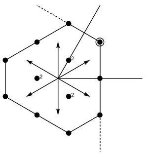
Standard basis

Root system of {SU(3). The 6 roots are mutually inclined by π/3 to form a hexagonal lattice: α corresponds to isospin; β to U-spin; and α+β to V-spin.

A slightly differently normalized standard basis consists of the F-spin operators, which are defined as Fi^=12λi{displaystyle {hat {F_{i}}}={frac {1}{2}}lambda _{i}} for the 3, and are utilized to apply to any representation of this algebra.

The Cartan–Weyl basis of the Lie algebra of SU(3) is obtained by another change of basis, where one defines,^[4]

I^±=F^1±iF^2{displaystyle {hat {I}}_{pm }={hat {F}}_{1}pm i{hat {F}}_{2}}

I^3=F3^{displaystyle {hat {I}}_{3}={hat {F_{3}}}}

V^±=F^4±iF^5{displaystyle {hat {V}}_{pm }={hat {F}}_{4}pm i{hat {F}}_{5}}

U^±=F^6±iF^7{displaystyle {hat {U}}_{pm }={hat {F}}_{6}pm i{hat {F}}_{7}}

Y^=23F^8 .{displaystyle {hat {Y}}={frac {2}{sqrt {3}}}{hat {F}}_{8}~.}

Because of the factors of i in these formulas, this is technically a basis for the complexification of the su(3) Lie algebra, namely sl(3,C). The preceding basis is then essentially the same one used in Hall's book.^[5]

Commutation algebra of the generators

The standard form of generators of the SU(3) group satisfies the commutation relations given below,

All other commutation relations follow from hermitian conjugation of these operators.

These commutation relations can be used to construct the irreducible representations of the SU(3) group.

The representations of the group lie in the 2-dimensional I₃−Y plane. Here, I^3{displaystyle {hat {I}}_{3}} stands for the z-component of Isospin and Y^{displaystyle {hat {Y}}} is the Hypercharge, and they comprise the (abelian) Cartan subalgebra of the full Lie algebra. The maximum number of mutually commuting generators of a Lie algebra is called its rank: SU(3) has rank 2. The remaining 6 generators, the ± ladder operators, correspond to the 6 roots arranged on the 2-dimensional hexagonal lattice of the figure.

Casimir operators

The Casimir operator is an operator that commutes with all the generators of the Lie group. In the case of SU(2), the quadratic operator J² is the only independent such operator.

In the case of SU(3) group, by contrast, two independent Casimir operators can be constructed, a quadratic and a cubic: they are,^[6]

C1^=∑kFk^Fk^{displaystyle {hat {C_{1}}}=sum _{k}{hat {F_{k}}}{hat {F_{k}}}}

C2^=∑jkldjklFj^Fk^Fl^ .{displaystyle {hat {C_{2}}}=sum _{jkl}d_{jkl}{hat {F_{j}}}{hat {F_{k}}}{hat {F_{l}}}~.}

These Casimir operators serve to label the irreducible representations of the Lie group algebra SU(3), because all states in a given representation assume the same value for each Casimir operator, which serves as the identity in a space with the dimension of that representation. This is because states in a given representation are connected by the action of the generators of the Lie algebra, and all generators commute with the Casimir operators.

For example, for the triplet representation, D(1,0), the eigenvalue of C^1{displaystyle {hat {C}}_{1}} is 4/3, and of C^2{displaystyle {hat {C}}_{2}}, 10/9.

More generally, from Freudenthal's formula, for generic D(p,q), the eigenvalue^[7] of C^1{displaystyle {hat {C}}_{1}} is (p2+q2+3p+3q+pq)/3{displaystyle (p^{2}+q^{2}+3p+3q+pq)/3}.

The eigenvalue ("anomaly coefficient") of C^2{displaystyle {hat {C}}_{2}} is^[8](p−q)(3+p+2q)(3+q+2p)/18.{displaystyle (p-q)(3+p+2q)(3+q+2p)/18.}
It is an odd function under the interchange p ↔ q. Consequently, it vanishes for real representations p=q, such as the adjoint, D(1,1), i.e. both C^2{displaystyle {hat {C}}_{2}} and anomalies vanish for it.

Representations of the SU(3) group

The irreducible representations of SU(3) are analyzed in various places, including Hall's book.^[9] Since the SU(3) group is simply connected,^[10] the representations are in one-to-one correspondence with the representations of its Lie algebra^[11] su(3), or the complexification^[12] of its Lie algebra, sl(3,C).

The representations are labeled as D(p,q), with p and q being non-negative integers, where in physical terms, p is the number of quarks and q is the number of antiquarks. Mathematically, the representation D(p,q) may be constructed by tensoring together p copies of the standard 3-dimensional representation and q copies of the dual of the standard representation, and then extracting an irreducible invariant subspace.^[13] (See also the section of Young tableaux below: p is the number of single-box columns, "quarks", and q the number of double-box columns, "antiquarks"). Still another way to think about the parameters p and q is as the maximum eigenvalues of the diagonal matrices

H1=(1000−10000),H2=(00001000−1){displaystyle H_{1}={begin{pmatrix}1&0&0\0&-1&0\0&0&0end{pmatrix}},quad H_{2}={begin{pmatrix}0&0&0\0&1&0\0&0&-1end{pmatrix}}}.

(The elements H1{displaystyle H_{1}} and H2{displaystyle H_{2}} are linear combinations of the elements I^3{displaystyle {hat {I}}_{3}} and Y^{displaystyle {hat {Y}}}, but normalized so that the eigenvalues of H1{displaystyle H_{1}} and H2{displaystyle H_{2}} are integers.)
This is to be compared to the representation theory of SU(2), where the irreducible representations are labeled by the maximum eigenvalue of a single element, h.

The representations have dimension^[14]

The 10 representation D(3,0) (spin 3/2 baryon decuplet)

d(p,q)=12(p+1)(q+1)(p+q+2).{displaystyle d(p,q)={frac {1}{2}}(p+1)(q+1)(p+q+2).}

An SU(3) multiplet may be completely specified by five labels, two of which, the eigenvalues of the two Casimirs, are common to all members of the multiplet. This generalizes the mere two labels for SU(2) multiplets, namely the eigenvalues of its quadratic Casimir and of I₃.

Since [I^3,Y^]=0{displaystyle [{hat {I}}_{3},{hat {Y}}]=0}, we can
label different states by the eigenvalues of I^3{displaystyle {hat {I}}_{3}} and Y^{displaystyle {hat {Y}}} operators, |t,y⟩{displaystyle |t,yrangle }, for a given eigenvalue of the isospin Casimir. The action of operators on this states are,^[15]

I^3|t,y⟩=t|t,y⟩{displaystyle {hat {I}}_{3}|t,yrangle =t|t,yrangle }

The representation of generators of the SU(3) group.

Y^|t,y⟩=y|t,y⟩{displaystyle {hat {Y}}|t,yrangle =y|t,yrangle }

U^0|t,y⟩=(34y−12t)|t,y⟩{displaystyle {hat {U}}_{0}|t,yrangle ={Bigl (}{frac {3}{4}}y-{frac {1}{2}}t{Bigr )}|t,yrangle }

V^0|t,y⟩=(34y+12t)|t,y⟩{displaystyle {hat {V}}_{0}|t,yrangle ={Bigl (}{frac {3}{4}}y+{frac {1}{2}}t{Bigr )}|t,yrangle }

I^±|t,y⟩=α|t±12,y⟩{displaystyle {hat {I}}_{pm }|t,yrangle =alpha |tpm {frac {1}{2}},yrangle }

U^±|t,y⟩=β|t±12,y±1⟩{displaystyle {hat {U}}_{pm }|t,yrangle =beta |tpm {frac {1}{2}},ypm 1rangle }

V^±|t,y⟩=γ|t∓12,y±1⟩{displaystyle {hat {V}}_{pm }|t,yrangle =gamma |tmp {frac {1}{2}},ypm 1rangle }

Here,

U^0≡12[U^+,U^−]=34Y^−12I^3{displaystyle {hat {U}}_{0}equiv {frac {1}{2}}[{hat {U}}_{+},{hat {U}}_{-}]={frac {3}{4}}{hat {Y}}-{frac {1}{2}}{hat {I}}_{3}}

and

V^0≡12[V^+,V^−]=34Y^+12I^3.{displaystyle {hat {V}}_{0}equiv {frac {1}{2}}[{hat {V}}_{+},{hat {V}}_{-}]={frac {3}{4}}{hat {Y}}+{frac {1}{2}}{hat {I}}_{3}.}

The 15-dimensional representation D(2,1)

All the other states of the representation can be constructed by the successive application of the ladder operators I^±,U^±{displaystyle {hat {I}}_{pm },{hat {U}}_{pm }} and V^±{displaystyle {hat {V}}_{pm }} and by identifying the base states which are annihilated by the action of the lowering operators. These operators lie on the vertices and the center of a hexagon.

Clebsch–Gordan coefficient for SU(3)

The product representation of two irreducible representations D(p1,q1){displaystyle D(p_{1},q_{1})} and D(p2,q2){displaystyle D(p_{2},q_{2})} is generally reducible. Symbolically,

D(p1,q1)⊗D(p2,q2)=∑P,Q⊕σ(P,Q)D(P,Q) ,{displaystyle D(p_{1},q_{1})otimes D(p_{2},q_{2})=sum _{P,Q}oplus sigma (P,Q)D(P,Q)~,}

where σ(P,Q){displaystyle sigma (P,Q)} is an integer.

For example, two octets (adjoints) compose to

D(1,1)⊗D(1,1)=D(2,2)⊕D(3,0)⊕D(1,1)⊕D(1,1)⊕D(0,3)⊕D(0,0) ,{displaystyle D(1,1)otimes D(1,1)=D(2,2)oplus D(3,0)oplus D(1,1)oplus D(1,1)oplus D(0,3)oplus D(0,0)~,}

that is, their product reduces to an icosaseptet (27), decuplet, two octets, an antidecuplet, and a singlet, 64 states in all.

The right-hand series is called the Clebsch–Gordan series. It implies that the representation D(P,Q){displaystyle D(P,Q)} appears σ(P,Q){displaystyle sigma (P,Q)} times in the reduction of this direct product of D(p1,q1){displaystyle D(p_{1},q_{1})} with D(p2,q2){displaystyle D(p_{2},q_{2})}.

Now a complete set of operators is needed to specify uniquely the states of each irreducible representation inside the one just reduced.
The complete set of commuting operators (CSCO) in the case of the irreducible representation D(P,Q){displaystyle D(P,Q)} is

{C^1,C^2,I^3,I^2,Y^} ,{displaystyle {{hat {C}}_{1},{hat {C}}_{2},{hat {I}}_{3},{hat {I}}^{2},{hat {Y}}}~,}

where

I2≡I12+I32+I32{displaystyle I^{2}equiv {I_{1}}^{2}+{I_{3}}^{2}+{I_{3}}^{2}}.

The states of the above direct product representation are thus completely represented by the set of operators

{C^1(1),C^2(1),I^3(1),I^2(1),Y^(1),C^1(2),C^2(2),I^3(2),I^2(2),Y^(2)},{displaystyle {{hat {C}}_{1}(1),{hat {C}}_{2}(1),{hat {I}}_{3}(1),{hat {I}}^{2}(1),{hat {Y}}(1),{hat {C}}_{1}(2),{hat {C}}_{2}(2),{hat {I}}_{3}(2),{hat {I}}^{2}(2),{hat {Y}}(2)},}

where the number in the parentheses designates the representation on which the operator acts.

An alternate set of commuting operators can be found for the direct product representation, if one considers the following set of operators,^[16]

C^1=C^1(1)+C^1(2)C^2=C^2(1)+C^2(2)I^2=I^2(1)+I^2(2)Y^=Y^(1)+Y^(2)I^3=I^3(1)+I^3(2).{displaystyle {begin{aligned}{hat {mathbb {C} }}_{1}&={hat {C}}_{1}(1)+{hat {C}}_{1}(2)\{hat {mathbb {C} }}_{2}&={hat {C}}_{2}(1)+{hat {C}}_{2}(2)\{hat {mathbb {I} }}^{2}&={hat {I}}^{2}(1)+{hat {I}}^{2}(2)\{hat {mathbb {Y} }}&={hat {Y}}(1)+{hat {Y}}(2)\{hat {mathbb {I} }}_{3}&={hat {I}}_{3}(1)+{hat {I}}_{3}(2).end{aligned}}}

Thus, the set of commuting operators includes

{C^1,C^2,Y^,I^3,I^2,C^1(1),C^1(2),C^2(1),C^2(2)}.{displaystyle {{hat {mathbb {C} }}_{1},{hat {mathbb {C} }}_{2},{hat {mathbb {Y} }},{hat {mathbb {I} }}_{3},{hat {mathbb {I} }}^{2},{hat {C}}_{1}(1),{hat {C}}_{1}(2),{hat {C}}_{2}(1),{hat {C}}_{2}(2)}.}

This is a set of nine operators only. But the set must contain ten operators to define all the states of the direct product representation uniquely. To find the last operator Γ, one must look outside the group. It is necessary to distinguish different D(P,Q){displaystyle D(P,Q)} for similar values of P and Q.

OperatorEigenvalueOperatorEigenvalueOperatorEigenvalueOperatorEigenvalueC^1(1)c11C^1(2)c12C^2(1)c21C^2(2)c22I^2i2I^3izY^yΓ^γC^1c1C^2c1Y^1y1Y^2y2I^2(1)i21I^2(2)i22I^3(1)iz1I^3(2)iz2{displaystyle {begin{array}{cc|cc|cc|cc}{text{Operator}}&{text{Eigenvalue}}&{text{Operator}}&{text{Eigenvalue}}&{text{Operator}}&{text{Eigenvalue}}&{text{Operator}}&{text{Eigenvalue}}\hline {hat {C}}_{1}(1)&{c^{1}}_{1}&{hat {C}}_{1}(2)&{c^{1}}_{2}&{hat {C}}_{2}(1)&{c^{2}}_{1}&{hat {C}}_{2}(2)&{c^{2}}_{2}\{hat {mathbb {I} }}^{2}&{i^{2}}&{hat {mathbb {I} }}_{3}&{i^{z}}&{hat {mathbb {Y} }}&{y}&{hat {Gamma }}&gamma \{hat {mathbb {C} }}_{1}&{c^{1}}&{hat {mathbb {C} }}_{2}&{c^{1}}&{hat {Y}}_{1}&{y}_{1}&{hat {Y}}_{2}&{y}_{2}\{hat {I}}^{2}(1)&{i^{2}}_{1}&{hat {I}}^{2}(2)&{i^{2}}_{2}&{hat {I}}_{3}(1)&{i^{z}}_{1}&{hat {I}}_{3}(2)&{i^{z}}_{2}end{array}}}

Thus, any state in the direct product representation can be represented by the ket,

|c11,c12,c21,c22,y1,y2,i21,i22,iz1,iz2⟩{displaystyle |{c^{1}}_{1},{c^{1}}_{2},{c^{2}}_{1},{c^{2}}_{2},y_{1},y_{2},{i^{2}}_{1},{i^{2}}_{2},{i^{z}}_{1},{i^{z}}_{2}rangle }

also using the second complete set of commuting operator, we can define the states in the direct product representation as

|c11,c12,c21,c22,y,γ,i2,iz,c1,c2⟩{displaystyle |{c^{1}}_{1},{c^{1}}_{2},{c^{2}}_{1},{c^{2}}_{2},y,gamma ,{i^{2}},{i^{z}},c^{1},c^{2}rangle }

We can drop the c11,c12,c21,c22{displaystyle {c^{1}}_{1},{c^{1}}_{2},{c^{2}}_{1},{c^{2}}_{2}} from the state and label the states as

|y1,y2,i21,i22,iz1,iz2⟩{displaystyle |y_{1},y_{2},{i^{2}}_{1},{i^{2}}_{2},{i^{z}}_{1},{i^{z}}_{2}rangle }

using the operators from the first set, and,

|y,γ,i2,iz,c1,c2⟩ ,{displaystyle |y,gamma ,{i^{2}},{i^{z}},c^{1},c^{2}rangle ~,}

using the operators from the second set.

Both these states span the direct product representation and any states in the representation can be labeled by suitable choice of the eigenvalues.

Using the completeness relation,

Here, the coefficients

are the Clebsch–Gordan coefficients.

A different notation

To avoid confusion, the eigenvalues c1,c2{displaystyle c^{1},c^{2}} can be simultaneously denoted by μ and the eigenvalues i2,iz,y{displaystyle i^{2},i^{z},y} are simultaneously denoted by ν. Then the eigenstate of the direct product representation D(P,Q){displaystyle D(P,Q)} can be denoted by^[16]

ψ(μ1μ2γν),{displaystyle psi {begin{pmatrix}mu _{1}&mu _{2}&gamma \&&nu end{pmatrix}},}

where μ1{displaystyle mu _{1}} is the eigenvalues of c11,c21{displaystyle {c^{1}}_{1},{c^{2}}_{1}} and μ2{displaystyle mu _{2}} is the eigenvalues of c12,c22{displaystyle {c^{1}}_{2},{c^{2}}_{2}} denoted simultaneously. Here, the quantity expressed by the parenthesis is the Wigner 3-j symbol.

Furthermore, ϕμ1ν1{displaystyle {phi ^{mu _{1}}}_{nu _{1}}} are considered to be the basis states of D(p1,q1){displaystyle D(p_{1},q_{1})} and ϕμ2ν2{displaystyle {phi ^{mu _{2}}}_{nu _{2}}} are the basis states of D(p2,q2){displaystyle D(p_{2},q_{2})}. Also ϕμ1ν1,ϕμ2ν2{displaystyle {phi ^{mu _{1}}}_{nu _{1}},{phi ^{mu _{2}}}_{nu _{2}}} are the basis states of the product representation. Here ν1,ν2{displaystyle nu _{1},nu _{2}} represents the combined eigenvalues (i21,iz1,y1){displaystyle ({i^{2}}_{1},{i^{z}}_{1},y_{1})} and (i22,iz2,y2){displaystyle ({i^{2}}_{2},{i^{z}}_{2},y_{2})} respectively.

Thus the unitary transformations that connects the two bases are

ψ(μ1μ2γν)=∑ν1,ν2(μ1μ2γν1ν2ν)ϕμ1ν1ϕμ2ν2{displaystyle psi {begin{pmatrix}mu _{1}&mu _{2}&gamma \&&nu end{pmatrix}}=sum _{nu _{1},nu _{2}}{begin{pmatrix}mu _{1}&mu _{2}&gamma \nu _{1}&nu _{2}&nu end{pmatrix}}{phi ^{mu _{1}}}_{nu _{1}}{phi ^{mu _{2}}}_{nu _{2}}}

This is a comparatively compact notation. Here,

(μ1μ2γν1ν2ν){displaystyle {begin{pmatrix}mu _{1}&mu _{2}&gamma \nu _{1}&nu _{2}&nu end{pmatrix}}}

are the Clebsch–Gordan coefficients.

Orthogonality relations

The Clebsch–Gordan coefficients form a real orthogonal matrix. Therefore,

ϕμ1ν1ϕμ2ν2=∑μ,ν,γ(μ1μ2γν1ν2ν)ψ(μ1μ2γν).{displaystyle {phi ^{mu _{1}}}_{nu _{1}}{phi ^{mu _{2}}}_{nu _{2}}=sum _{mu ,nu ,gamma }{begin{pmatrix}mu _{1}&mu _{2}&gamma \nu _{1}&nu _{2}&nu end{pmatrix}}psi {begin{pmatrix}mu _{1}&mu _{2}&gamma \&&nu end{pmatrix}}.}

Also, they follow the following orthogonality relations,

∑ν1,ν2(μ1μ2γν1ν2ν)(μ1μ2γ′ν1ν2ν′)=δνν′δγ,γ′{displaystyle sum _{nu _{1},nu _{2}}{begin{pmatrix}mu _{1}&mu _{2}&gamma \nu _{1}&nu _{2}&nu end{pmatrix}}{begin{pmatrix}mu _{1}&mu _{2}&gamma '\nu _{1}&nu _{2}&nu 'end{pmatrix}}=delta _{nu nu '}delta _{gamma ,gamma '}}

∑μνγ(μ1μ2γν1ν2ν)(μ1μ2γν1′ν2′ν)=δν1ν1′δν2,ν2′{displaystyle sum _{mu nu gamma }{begin{pmatrix}mu _{1}&mu _{2}&gamma \nu _{1}&nu _{2}&nu end{pmatrix}}{begin{pmatrix}mu _{1}&mu _{2}&gamma \nu _{1}'&nu _{2}'&nu end{pmatrix}}=delta _{nu _{1}nu _{1}'}delta _{nu _{2},nu _{2}'}}

Symmetry properties

If an irreducible representation μγ{displaystyle {scriptstyle {mu }_{gamma }}} apperars in the Clebsch–Gordan series of μ1⊗μ2{displaystyle {scriptstyle {mu }_{1}otimes {mu }_{2}}}, then it must appear in the Clebsch–Gordan series of μ2⊗μ1{displaystyle {scriptstyle {mu }_{2}otimes {mu }_{1}}}. Which implies,

(μ1μ2γν1ν2ν)=ξ1(μ2μ1γν2ν1ν){displaystyle {begin{pmatrix}mu _{1}&mu _{2}&gamma \nu _{1}&nu _{2}&nu end{pmatrix}}=xi _{1}{begin{pmatrix}mu _{2}&mu _{1}&gamma \nu _{2}&nu _{1}&nu end{pmatrix}}}

Where ξ1=ξ1(μ1,μ2,γ)=±1{displaystyle xi _{1}=xi _{1}(mu _{1},mu _{2},gamma )=pm 1}

Since the Clebsch–Gordan coefficients are all real, the following symmetry property can be deduced,

(μ1μ2γν1ν2ν)=ξ2(μ1∗μ2∗γ∗ν1ν2ν){displaystyle {begin{pmatrix}mu _{1}&mu _{2}&gamma \nu _{1}&nu _{2}&nu end{pmatrix}}=xi _{2}{begin{pmatrix}{mu _{1}}^{*}&{mu _{2}}^{*}&{gamma }^{*}\nu _{1}&nu _{2}&nu end{pmatrix}}}

Where ξ2=ξ2(μ1,μ2,γ)=±1{displaystyle xi _{2}=xi _{2}(mu _{1},mu _{2},gamma )=pm 1}.

Symmetry group of the 3D oscillator Hamiltonian operator

A three-dimensional harmonic oscillator is described by the Hamiltonian

H^=−12∇2+12(x2+y2+z2),{displaystyle {hat {H}}=-{frac {1}{2}}nabla ^{2}+{frac {1}{2}}(x^{2}+y^{2}+z^{2}),}

where the spring constant, the mass and Planck's constant have been absorbed into the definition of the variables, ħ=m=1.

It is seen that this Hamiltonian is symmetric under coordinate transformations that preserve the value of V=x2+y2+z2{displaystyle V=x^{2}+y^{2}+z^{2}}. Thus, any operators in the group SO(3) keep this Hamiltonian invariant.

More significantly, since the Hamiltonian is Hermitian, it further remains invariant under operation by elements of the much larger SU(3) group.

More systematically, operators such as the Ladder operators

2ai^=Xi^+iPi^  {displaystyle {sqrt {2}}{hat {a_{i}}}={hat {X_{i}}}+i{hat {P_{i}}}~~} and   2ai^†=Xi^+iPi^{displaystyle ~~{sqrt {2}}{hat {a_{i}}}^{dagger }={hat {X_{i}}}+i{hat {P_{i}}}}

can be constructed which raise and lower the eigenvalue of the Hamiltonian operator by 1.

The operators â_i and â_i^† are not hermitian; but hermitian operators can be constructed from different combinations of them,

namely,   ai^aj^†{displaystyle {hat {a_{i}}}{hat {a_{j}}}^{dagger }}.

There are nine such operators for i,j=1,2,3.

The nine hermitian operators formed by the bilinear forms â_i^†â_j are controlled by the fundamental commutators

[ai^,aj^†]=δij,{displaystyle [{hat {a_{i}}},{hat {a_{j}}}^{dagger }]=delta _{ij},}

[ai^,aj^]=[ai^†,aj^†]=0,{displaystyle [{hat {a_{i}}},{hat {a_{j}}}]=[{hat {a_{i}}}^{dagger },{hat {a_{j}}}^{dagger }]=0,}

and seen to not commute among themselves. As a result, this complete set of operators don't share their eigenvectors in common, and they cannot be diagonalized simultaneously. The group is thus non-Abelian and degeneracies may be present in the Hamiltonian, as indicated.

The Hamiltonian of the 3D isotropic harmonic oscillator, when written in terms of the operator Ni^=ai^†ai^{displaystyle {hat {N_{i}}}={hat {a_{i}}}^{dagger }{hat {a_{i}}}} amounts to

H^=ω[32+N1^+N2^+N3^]{displaystyle {hat {H}}=omega left[{frac {3}{2}}+{hat {N_{1}}}+{hat {N_{2}}}+{hat {N_{3}}}right]}.

The Hamiltonian has 8-fold degeneracy. A successive application of â_i and â_j^† on the left preserves the Hamiltonian invariant, since it increases N_i by 1 and decrease N_j by 1, thereby keeping the total

N=∑Ni{displaystyle N=sum {N_{i}}}   constant. (cf. quantum harmonic oscillator)

The maximally commuting set of operators

Since the operators belonging to the symmetry group of Hamiltonian do not always form an Abelian group, a common eigenbasis cannot be found that diagonalizes all of them simultaneously. Instead, we take the maximally commuting set of operators from the symmetry group of the Hamiltonian, and try to reduce the matrix representations of the group into irreducible representations.

Hilbert space of two systems

The Hilbert space of two particles is the tensor product of the two Hilbert spaces of the two individual particles,

H=H1⊗I+I⊗H2 ,{displaystyle mathbb {H} =mathbb {H} _{1}otimes mathbb {I} +mathbb {I} otimes mathbb {H} _{2}~,}

where H1{displaystyle mathbb {H} _{1}} and H2{displaystyle mathbb {H} _{2}} are the Hilbert space of the first and second particles, respectively.

The operators in each of the Hilbert spaces have their own commutation relations, and an operator of one Hilbert space commutes with an operator from the other Hilbert space. Thus the symmetry group of the two particle Hamiltonian operator is the superset of the symmetry groups of the Hamiltonian operators of individual particles. If the individual Hilbert spaces are N dimensional, the combined Hilbert space is N² dimensional.

Clebsch–Gordan coefficient in this case

The symmetry group of the Hamiltonian is SU(3). As a result, the Clebsch–Gordan coefficients can be found by expanding the uncoupled basis vectors of the symmetry group of the Hamiltonian into its coupled basis. The Clebsch–Gordan series is obtained by block-diagonalizing the Hamiltonian through the unitary transformation constructed from the eigenstates which diagonalizes the maximal set of commuting operators.

Young tableaux

A Young tableau (plural tableaux) is a method for decomposing products of an SU(N) group representation into a sum of irreducible representations. It provides the dimension and symmetry types of the irreducible representations, which is known as the Clebsch–Gordan series. Each irreducible representation corresponds to a single-particle state and a product of more than one irreducible representation indicates a multiparticle state.

Since the particles are mostly indistinguishable in quantum mechanics, this approximately relates to several permutable particles. The permutations of n identical particles constitute the symmetric group S_n. Every n-particle state of S_n that is made up of single-particle states of the fundamental N-dimensional SU(N) multiplet belongs to an irreducible SU(N) representation. Thus, it can be used to determine the Clebsch–Gordan series for any unitary group.^[18]

Constructing the states

Any two particle wavefunctionψ1,2{displaystyle psi _{1,2}}, where the indices 1,2 represents the state of particle 1 and 2, can be used to generate states of explicit symmetry using the symmetrizing and the anti-symmetrizing operators.^[19]

S12=I+P12{displaystyle mathbf {S_{12}} =mathbf {I} +mathbf {P_{12}} }

A12=I−P12{displaystyle mathbf {A_{12}} =mathbf {I} -mathbf {P_{12}} }

where the P12{displaystyle mathbf {P_{12}} } are the operator that interchanges the particles (Exchange operator).

The following relation follows:^[19]-

P12P12=I{displaystyle mathbf {P_{12}P_{12}} =mathbf {I} }

P12S12=P12+I=S12{displaystyle mathbf {P_{12}S_{12}} =mathbf {P_{12}} +mathbf {I} =mathbf {S_{12}} }

P12A12=P12−I=−A12{displaystyle mathbf {P_{12}A_{12}} =mathbf {P_{12}} -mathbf {I} =-mathbf {A_{12}} }

P12S12ψ12=+S12ψ12{displaystyle mathbf {P_{12}} mathbf {S_{12}} psi _{12}=+mathbf {S_{12}} psi _{12}}

thus,

P12A12ψ12=−A12ψ12.{displaystyle mathbf {P_{12}} mathbf {A_{12}} psi _{12}=-mathbf {A_{12}} psi _{12}.}

Starting from a multipartice state, we can apply S12{displaystyle mathbf {S_{12}} } and A12{displaystyle mathbf {A_{12}} } repeatedly to construct states that are:^[19]-

1. Symmetric with respect to all particles.


2. Antisymmetric with respect to all particles.


3. Mixed symmetries, i.e. symmetric or antisymmetric with respect to some particles.

Constructing the tableaux

Instead of using ψ, in Young tableaux, we use square boxes (□) to denote particles and i to denote the state of the particles.

A sample Young tableau. The number inside the boxes represents the state of the particles

The complete set of np{displaystyle n_{p}} particles are denoted by arrangements of np{displaystyle n_{p}} □s, each with its own quantum number label (i).

The tableaux is formed by stacking boxes side by side by side and up-down such that the states symmetrised with respect to all particles are given ia a row and the states anti-symmetrised with respect to all particles lies in a single column. Following rules are followed while constructing the tableaux:^[18]

1. A row must not be longer than the one before it.


2. The quantum labels (numbers in the □) should not decrease while going left to right in a row.


3. The quantum labels must strictly increase while going down in a column.

Case for N = 3

For N=3 that is in the case of SU(3), the following situation arises. In SU(3) there are three labels, they are generally designated by (u,d,s) corresponding to up, down and strange quarks which follows the SU(3) algebra. They can also be designated generically as (1,2,3). For two particle system, we have the following six symmetry states:

11uu{displaystyle {{begin{array}{|c|c|}hline 1&1\hline end{array}} atop uu}}

1212(ud+du){displaystyle {{begin{array}{|c|c|}hline 1&2\hline end{array}} atop {frac {1}{sqrt {2}}}(ud+du)}}

1312(us+su){displaystyle {{begin{array}{|c|c|}hline 1&3\hline end{array}} atop {frac {1}{sqrt {2}}}(us+su)}}

22dd{displaystyle {{begin{array}{|c|c|}hline 2&2\hline end{array}} atop dd}}

2312(ds+sd){displaystyle {{begin{array}{|c|c|}hline 2&3\hline end{array}} atop {frac {1}{sqrt {2}}}(ds+sd)}}

33ss{displaystyle {{begin{array}{|c|c|}hline 3&3\hline end{array}} atop ss}}

and the following three antisymmetric states:

1212(ud−du)1312(us−su)2312(ds−sd){displaystyle {{begin{array}{|c|}hline 1\hline 2\hline end{array}} atop {frac {1}{sqrt {2}}}(ud-du)}qquad {{begin{array}{|c|}hline 1\hline 3\hline end{array}} atop {frac {1}{sqrt {2}}}(us-su)}qquad {{begin{array}{|c|}hline 2\hline 3\hline end{array}} atop {frac {1}{sqrt {2}}}(ds-sd)}}

The 1-column, 3-row tableau is the singlet, and so all tableaux of nontrivial irreps of SU(3) cannot have more than two rows. The representation D(p,q) has
p+q boxes on the top row and q boxes on the second row.

Clebsch–Gordan series from the tableaux

Clebsch–Gordan series is the expansion of the direct product of two irreducible representation into direct sum of irreducible representations.
D(p1,q1)⊗D(p2,q2)=∑P,Q⊕D(P,Q){displaystyle D(p_{1},q_{1})otimes D(p_{2},q_{2})=sum _{P,Q}oplus D(P,Q)}. This can be easily found out from the Young tableaux.

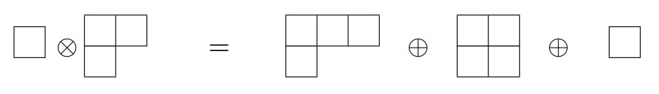
Procedure to obtain the Clebsch–Gordan series from Young tableaux:

The following steps are followed to construct the Clebsch–Gordan series from the Young tableaux:[20] Write down the two Young diagrams for the two irreps under consideration, such as in the following example. In the second figure insert a series of the letter a in the first row, the letter b in the second row, the letter c in the third row, etc. in order to keep track of them once they are included in the various resultant diagrams: Take the first box containing an a and appends it to the first Young diagram in all possible ways that follow the rules for creation of a Young diagram: Then take the next box containing an a and do the same thing with it, except that we are not allowed to put two a's together in the same column. The last diagram in the curly bracket contains two a in the same column thus the diagram must be deleted. Thereby giving: Append the last box to the diagram in curly bracket in all possible ways resulting in: In each rows while counting from right to left, if at any point the number of a particular alphabet encountered be more than the number of the previous alphabet, then the diagram must be deleted. Here the first and the third diagram should be deleted, resulting in:

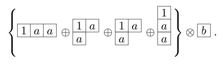
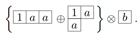
Example of Clebsch–Gordan series for SU(3)

The tensor product of a triplet with an octet reducing to a deciquintuplet (15), an anti-sextet, and a triplet

D(1,0)⊗D(1,1)=D(2,1)⊕D(0,2)⊕D(1,0){displaystyle D(1,0)otimes D(1,1)=D(2,1)oplus D(0,2)oplus D(1,0)}

appears diagrammatically as^[20]-

a total of 24 states.
Using the same procedure, any direct product representation is easily reduced.

See also

• Wigner D-matrix


• Tensor operator


• Wigner-Eckart theorem


• Representation theory


• Racah W-coefficient


• Gell-Mann–Okubo mass formula

References

• 
  Greiner, W.; Müller, B. (1994). Quantum Mechanics: Symmetries (2nd ed.). Springer. ISBN 978-3540580805.
  


• 
  Hall, Brian C. (2015), Lie Groups, Lie Algebras, and Representations: An Elementary Introduction, Graduate Texts in Mathematics, 222 (2nd ed.), Springer, ISBN 978-3319134666
  


• 
  McNamee, P.; j., S.; Chilton, F. (1964). "Tables of Clebsch-Gordan Coefficients of SU3". Reviews of Modern Physics. 36 (4): 1005. Bibcode:1964RvMP...36.1005M. doi:10.1103/RevModPhys.36.1005.
  


• 
  Mandel'tsveig, V. B. (1965). "Irreducible representations of the SU3 group". Sov Phys JETP. 20 (5): 1237–1243.
  online
  

External links

• – Clebsch–Gordan coefficients for SU(3) using simple symmetries