Fourier transform
The Fourier transform (FT) decomposes a function of time (a signal) into the frequencies that make it up, in a way similar to how a musical chord can be expressed as the frequencies (or pitches) of its constituent notes. The Fourier transform of a function of time is itself a complex-valued function of frequency, whose absolute value represents the amount of that frequency present in the original function, and whose complex argument is the phase offset of the basic sinusoid in that frequency. The Fourier transform is called the frequency domain representation of the original signal. The term Fourier transform refers to both the frequency domain representation and the mathematical operation that associates the frequency domain representation to a function of time. The Fourier transform is not limited to functions of time, but in order to have a unified language, the domain of the original function is commonly referred to as the time domain. For many functions of practical interest, one can define an operation that reverses this: the inverse Fourier transformation, also called Fourier synthesis, of a frequency domain representation combines the contributions of all the different frequencies to recover the original function of time.
.mw-parser-output .mod-gallery{display:table}.mw-parser-output .mod-gallery-default{background:transparent;margin-top:0.5em}.mw-parser-output .mod-gallery-center{margin-left:auto;margin-right:auto}.mw-parser-output .mod-gallery-left{float:left}.mw-parser-output .mod-gallery-right{float:right}.mw-parser-output .mod-gallery-none{float:none}.mw-parser-output .mod-gallery-collapsible{width:100%}.mw-parser-output .mod-gallery .title{display:table-row}.mw-parser-output .mod-gallery .title>div{display:table-cell;text-align:center;font-weight:bold}.mw-parser-output .mod-gallery .main{display:table-row}.mw-parser-output .mod-gallery .main>div{display:table-cell}.mw-parser-output .mod-gallery .caption{display:table-row;vertical-align:top}.mw-parser-output .mod-gallery .caption>div{display:table-cell;display:block;font-size:94%;padding:0}.mw-parser-output .mod-gallery .footer{display:table-row}.mw-parser-output .mod-gallery .footer>div{display:table-cell;text-align:right;font-size:80%;line-height:1em}.mw-parser-output .mod-gallery .gallerybox .thumb img{background:none}.mw-parser-output .mod-gallery .bordered-images img{border:solid #eee 1px}.mw-parser-output .mod-gallery .whitebg img{background:#fff!important}.mw-parser-output .mod-gallery .gallerybox div{background:#fff!important}

A sinusoidal curve, with peak amplitude (1).
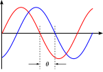
Illustration of phase shift θ.


Fourier transforms |
|---|
Continuous Fourier transform |
Fourier series |
Discrete-time Fourier transform |
Discrete Fourier transform |
Discrete Fourier transform over a ring |
Fourier analysis |
Related transforms |
Linear operations performed in one domain (time or frequency) have corresponding operations in the other domain, which are sometimes easier to perform. The operation of differentiation in the time domain corresponds to multiplication by the frequency,[remark 1] so some differential equations are easier to analyze in the frequency domain. Also, convolution in the time domain corresponds to ordinary multiplication in the frequency domain. Concretely, this means that any linear time-invariant system, such as a filter applied to a signal, can be expressed relatively simply as an operation on frequencies.[remark 2] After performing the desired operations, transformation of the result can be made back to the time domain. Harmonic analysis is the systematic study of the relationship between the frequency and time domains, including the kinds of functions or operations that are "simpler" in one or the other, and has deep connections to many areas of modern mathematics.
Functions that are localized in the time domain have Fourier transforms that are spread out across the frequency domain and vice versa, a phenomenon known as the uncertainty principle. The critical case for this principle is the Gaussian function, of substantial importance in probability theory and statistics as well as in the study of physical phenomena exhibiting normal distribution (e.g., diffusion). The Fourier transform of a Gaussian function is another Gaussian function. Joseph Fourier introduced the transform in his study of heat transfer, where Gaussian functions appear as solutions of the heat equation.
The Fourier transform can be formally defined as an improper Riemann integral, making it an integral transform, although this definition is not suitable for many applications requiring a more sophisticated integration theory.[remark 3] For example, many relatively simple applications use the Dirac delta function, which can be treated formally as if it were a function, but the justification requires a mathematically more sophisticated viewpoint.[remark 4] The Fourier transform can also be generalized to functions of several variables on Euclidean space, sending a function of 3-dimensional space to a function of 3-dimensional momentum (or a function of space and time to a function of 4-momentum). This idea makes the spatial Fourier transform very natural in the study of waves, as well as in quantum mechanics, where it is important to be able to represent wave solutions as functions of either space or momentum and sometimes both. In general, functions to which Fourier methods are applicable are complex-valued, and possibly vector-valued.[remark 5] Still further generalization is possible to functions on groups, which, besides the original Fourier transform on ℝ or ℝn (viewed as groups under addition), notably includes the discrete-time Fourier transform (DTFT, group = ℤ), the discrete Fourier transform (DFT, group = ℤ mod N) and the Fourier series or circular Fourier transform (group = S1, the unit circle ≈ closed finite interval with endpoints identified). The latter is routinely employed to handle periodic functions. The fast Fourier transform (FFT) is an algorithm for computing the DFT.
Contents
1 Definition
2 History
3 Introduction
4 Example
5 Properties of the Fourier transform
5.1 Basic properties
5.1.1 Linearity
5.1.2 Translation / time shifting
5.1.3 Modulation / frequency shifting
5.1.4 Time scaling
5.1.5 Conjugation
5.1.6 Real and imaginary part in time
5.1.7 Integration
5.2 Invertibility and periodicity
5.3 Units and duality
5.4 Uniform continuity and the Riemann–Lebesgue lemma
5.5 Plancherel theorem and Parseval's theorem
5.6 Poisson summation formula
5.7 Differentiation
5.8 Convolution theorem
5.9 Cross-correlation theorem
5.10 Eigenfunctions
5.11 Connection with the Heisenberg group
6 Complex domain
6.1 Laplace transform
6.2 Inversion
7 Fourier transform on Euclidean space
7.1 Uncertainty principle
7.2 Sine and cosine transforms
7.3 Spherical harmonics
7.4 Restriction problems
8 Fourier transform on function spaces
8.1 On Lp spaces
8.1.1 On L1
8.1.2 On L2
8.1.3 On other Lp
8.2 Tempered distributions
9 Generalizations
9.1 Fourier–Stieltjes transform
9.2 Locally compact abelian groups
9.3 Gelfand transform
9.4 Compact non-abelian groups
10 Alternatives
11 Applications
11.1 Analysis of differential equations
11.2 Fourier transform spectroscopy
11.3 Quantum mechanics
11.4 Signal processing
12 Other notations
13 Other conventions
14 Computation methods
14.1 Numerical integration of closed-form functions
14.2 Numerical integration of a series of ordered pairs
14.3 Discrete Fourier transforms and fast Fourier transforms
15 Tables of important Fourier transforms
15.1 Functional relationships, one-dimensional
15.2 Square-integrable functions, one-dimensional
15.3 Distributions, one-dimensional
15.4 Two-dimensional functions
15.5 Formulas for general n-dimensional functions
16 See also
17 Remarks
18 Notes
19 References
20 External links
Definition
The Fourier transform of the function f is traditionally denoted by adding a circumflex: f^{displaystyle {hat {f}}}

|

for any real number ξ.
The reason for the negative sign convention in the exponent is that in electrical engineering, it is common[3] to use f(x)=e2πiξ0x{displaystyle f(x)=e^{2pi ixi _{0}x}}


When the independent variable x represents time, the transform variable ξ represents frequency (e.g. if time is measured in seconds, then the frequency is in hertz). Under suitable conditions, f is determined by f^{displaystyle {hat {f}}}
|

for any real number x.
The statement that f can be reconstructed from f^{displaystyle {hat {f}}}
For other common conventions and notations, including using the angular frequency ω instead of the frequency ξ, see Other conventions and Other notations below. The Fourier transform on Euclidean space is treated separately, in which the variable x often represents position and ξ momentum. The conventions chosen in this article are those of harmonic analysis, and are characterized as the unique conventions such that the Fourier transform is both unitary on L2 and an algebra homomorphism from L1 to L∞, without renormalizing the Lebesgue measure.[9]
Many other characterizations of the Fourier transform exist. For example, one uses the Stone–von Neumann theorem: the Fourier transform is the unique unitary intertwiner for the symplectic and Euclidean Schrödinger representations of the Heisenberg group.
History
In 1822, Joseph Fourier showed that some functions could be written as an infinite sum of harmonics.[10]
Introduction
One motivation for the Fourier transform comes from the study of Fourier series. In the study of Fourier series, complicated but periodic functions are written as the sum of simple waves mathematically represented by sines and cosines. The Fourier transform is an extension of the Fourier series that results when the period of the represented function is lengthened and allowed to approach infinity.[11]
Due to the properties of sine and cosine, it is possible to recover the amplitude of each wave in a Fourier series using an integral. In many cases it is desirable to use Euler's formula, which states that e2πiθ = cos(2πθ) + i sin(2πθ), to write Fourier series in terms of the basic waves e2πiθ. This has the advantage of simplifying many of the formulas involved, and provides a formulation for Fourier series that more closely resembles the definition followed in this article. Re-writing sines and cosines as complex exponentials makes it necessary for the Fourier coefficients to be complex valued. The usual interpretation of this complex number is that it gives both the amplitude (or size) of the wave present in the function and the phase (or the initial angle) of the wave. These complex exponentials sometimes contain negative "frequencies". If θ is measured in seconds, then the waves e2πiθ and e−2πiθ both complete one cycle per second, but they represent different frequencies in the Fourier transform. Hence, frequency no longer measures the number of cycles per unit time, but is still closely related.
There is a close connection between the definition of Fourier series and the Fourier transform for functions f that are zero outside an interval. For such a function, we can calculate its Fourier series on any interval that includes the points where f is not identically zero. The Fourier transform is also defined for such a function. As we increase the length of the interval on which we calculate the Fourier series, then the Fourier series coefficients begin to look like the Fourier transform and the sum of the Fourier series of f begins to look like the inverse Fourier transform. To explain this more precisely, suppose that T is large enough so that the interval [−T/2, T/2] contains the interval on which f is not identically zero. Then the nth series coefficient cn is given by:
- cn=1T∫−T2T2f(x)e−2πi(nT)xdx.{displaystyle c_{n}={frac {1}{T}}int _{-{frac {T}{2}}}^{frac {T}{2}}f(x),e^{-2pi ileft({frac {n}{T}}right)x},dx.}

Comparing this to the definition of the Fourier transform, it follows that
- cn=1Tf^(nT){displaystyle c_{n}={frac {1}{T}}{hat {f}}left({frac {n}{T}}right)}

since f (x) is zero outside [−T/2, T/2]. Thus the Fourier coefficients are just the values of the Fourier transform sampled on a grid of width 1/T, multiplied by the grid width 1/T.
Under appropriate conditions, the Fourier series of f will equal the function f. In other words, f can be written:
- f(x)=∑n=−∞∞cne2πi(nT)x=∑n=−∞∞f^(ξn) e2πiξnxΔξ,{displaystyle f(x)=sum _{n=-infty }^{infty }c_{n},e^{2pi ileft({frac {n}{T}}right)x}=sum _{n=-infty }^{infty }{hat {f}}(xi _{n}) e^{2pi ixi _{n}x}Delta xi ,}

where the last sum is simply the first sum rewritten using the definitions ξn = n/T, and Δξ = n + 1/T − n/T = 1/T.
This second sum is a Riemann sum, and so by letting T → ∞ it will converge to the integral for the inverse Fourier transform given in the definition section. Under suitable conditions, this argument may be made precise.[12]
In the study of Fourier series the numbers cn could be thought of as the "amount" of the wave present in the Fourier series of f. Similarly, as seen above, the Fourier transform can be thought of as a function that measures how much of each individual frequency is present in our function f, and we can recombine these waves by using an integral (or "continuous sum") to reproduce the original function.
Example
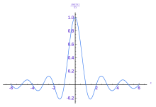
The following figures provide a visual illustration how the Fourier transform measures whether a frequency is present in a particular function. The depicted function f (t) = cos(6πt) e−πt2 oscillates at 3 Hz (if t measures seconds) and tends quickly to 0. (The second factor in this equation is an envelope function that shapes the continuous sinusoid into a short pulse. Its general form is a Gaussian function). This function was specially chosen to have a real Fourier transform that can easily be plotted. The first image contains its graph. In order to calculate f̂ (3) we must integrate e−2πi(3t)f (t). The second image shows the plot of the real and imaginary parts of this function. The real part of the integrand is almost always positive, because when f (t) is negative, the real part of e−2πi(3t) is negative as well. Because they oscillate at the same rate, when f (t) is positive, so is the real part of e−2πi(3t). The result is that when you integrate the real part of the integrand you get a relatively large number (in this case 1/2). On the other hand, when you try to measure a frequency that is not present, as in the case when we look at f̂ (5), you see that both real and imaginary component of this function vary rapidly between positive and negative values, as plotted in the third image. Therefore, in this case, the integrand oscillates fast enough so that the integral is very small and the value for the Fourier transform for that frequency is nearly zero.
The general situation may be a bit more complicated than this, but this in spirit is how the Fourier transform measures how much of an individual frequency is present in a function f (t).

Original function showing oscillation 3 Hz.
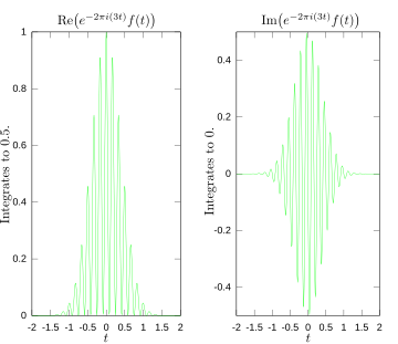
Real and imaginary parts of integrand for Fourier transform at 3 Hz
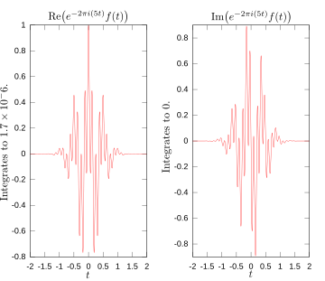
Real and imaginary parts of integrand for Fourier transform at 5 Hz

Magnitude of Fourier transform, with 3 and 5 Hz labeled.


Properties of the Fourier transform
Here we assume f (x), g(x) and h(x) are integrable functions: Lebesgue-measurable on the real line satisfying:
- ∫−∞∞|f(x)|dx<∞.{displaystyle int _{-infty }^{infty }|f(x)|,dx<infty .}

We denote the Fourier transforms of these functions as f̂ (ξ), ĝ(ξ) and ĥ(ξ) respectively.
Basic properties
The Fourier transform has the following basic properties:[13]
Linearity
- For any complex numbers a and b, if h(x) = af (x) + bg(x), then ĥ(ξ) = a · f̂ (ξ) + b · ĝ(ξ).
Translation / time shifting
- For any real number x0, if h(x) = f (x − x0), then ĥ(ξ) = e−2πix0ξf̂ (ξ).
Modulation / frequency shifting
- For any real number ξ0, if h(x) = e2πixξ0f (x), then ĥ(ξ) = f̂ (ξ − ξ0).
Time scaling
- For a non-zero real number a, if h(x) = f (ax), then
- h^(ξ)=1|a|f^(ξa).{displaystyle {hat {h}}(xi )={frac {1}{|a|}}{hat {f}}left({frac {xi }{a}}right).}
- h^(ξ)=1|a|f^(ξa).{displaystyle {hat {h}}(xi )={frac {1}{|a|}}{hat {f}}left({frac {xi }{a}}right).}
- The case a = −1 leads to the time-reversal property, which states: if h(x) = f (−x), then ĥ(ξ) = f̂ (−ξ).

Conjugation
- If h(x) = f (x), then
- h^(ξ)=f^(−ξ)¯.{displaystyle {hat {h}}(xi )={overline {{hat {f}}(-xi )}}.}
- h^(ξ)=f^(−ξ)¯.{displaystyle {hat {h}}(xi )={overline {{hat {f}}(-xi )}}.}
- In particular, if f is real, then one has the reality condition
- f^(−ξ)=f^(ξ)¯,{displaystyle {hat {f}}(-xi )={overline {{hat {f}}(xi )}},}
- f^(−ξ)=f^(ξ)¯,{displaystyle {hat {f}}(-xi )={overline {{hat {f}}(xi )}},}
- that is, f̂ is a Hermitian function. And if f is purely imaginary, then
- f^(−ξ)=−f^(ξ)¯.{displaystyle {hat {f}}(-xi )=-{overline {{hat {f}}(xi )}}.}
- f^(−ξ)=−f^(ξ)¯.{displaystyle {hat {f}}(-xi )=-{overline {{hat {f}}(xi )}}.}


Real and imaginary part in time
- If h(x)=ℜ(f(x)){displaystyle h(x)=Re {(f(x))}}
, then h^(ξ)=12(f^(ξ)+f^(−ξ)¯){displaystyle {hat {h}}(xi )={frac {1}{2}}({hat {f}}(xi )+{overline {{hat {f}}(-xi )}})}
.
- If h(x)=ℑ(f(x)){displaystyle h(x)=Im {(f(x))}}
, then h^(ξ)=12i(f^(ξ)−f^(−ξ)¯){displaystyle {hat {h}}(xi )={frac {1}{2i}}({hat {f}}(xi )-{overline {{hat {f}}(-xi )}})}
.
Integration
- Substituting ξ = 0 in the definition, we obtain
- f^(0)=∫−∞∞f(x)dx.{displaystyle {hat {f}}(0)=int _{-infty }^{infty }f(x),dx.}
- f^(0)=∫−∞∞f(x)dx.{displaystyle {hat {f}}(0)=int _{-infty }^{infty }f(x),dx.}
- That is, the evaluation of the Fourier transform at the origin (ξ = 0) equals the integral of f over all its domain.

Invertibility and periodicity
Under suitable conditions on the function f, it can be recovered from its Fourier transform f^{displaystyle {hat {f}}}
More precisely, defining the parity operator P that inverts time, P[ f ] : t ↦ f (−t):
- F0=Id,F1=F,F2=P,F4=Id,F3=F−1=P∘F=F∘P{displaystyle {begin{aligned}{mathcal {F}}^{0}&=mathrm {Id} ,quad {mathcal {F}}^{1}={mathcal {F}},\{mathcal {F}}^{2}&={mathcal {P}},quad {mathcal {F}}^{4}=mathrm {Id} ,\{mathcal {F}}^{3}&={mathcal {F}}^{-1}={mathcal {P}}circ {mathcal {F}}={mathcal {F}}circ {mathcal {P}}end{aligned}}}

These equalities of operators require careful definition of the space of functions in question, defining equality of functions (equality at every point? equality almost everywhere?) and defining equality of operators – that is, defining the topology on the function space and operator space in question. These are not true for all functions, but are true under various conditions, which are the content of the various forms of the Fourier inversion theorem.
This fourfold periodicity of the Fourier transform is similar to a rotation of the plane by 90°, particularly as the two-fold iteration yields a reversal, and in fact this analogy can be made precise. While the Fourier transform can simply be interpreted as switching the time domain and the frequency domain, with the inverse Fourier transform switching them back, more geometrically it can be interpreted as a rotation by 90° in the time–frequency domain (considering time as the x-axis and frequency as the y-axis), and the Fourier transform can be generalized to the fractional Fourier transform, which involves rotations by other angles. This can be further generalized to linear canonical transformations, which can be visualized as the action of the special linear group SL2(ℝ) on the time–frequency plane, with the preserved symplectic form corresponding to the uncertainty principle, below. This approach is particularly studied in signal processing, under time–frequency analysis.
Units and duality
In mathematics, one often does not think of any units as being attached to the two variables t and ξ. But in physical applications, ξ must have inverse units to the units of t. For example, if t is measured in seconds, ξ
should be in cycles per second for the formulas here to be valid. If the scale of t is changed and t is measured in units of 2π seconds, then either ξ must be in the so-called "angular frequency", or one must insert some constant scale factor into some of the formulas. If t is measured in units of length, then ξ must be in inverse length, e.g., wavenumbers. That is to say, there are two copies of the real line: one measured in one set of units, where t ranges, and the other in inverse units to the units of t, and which is the range of ξ. So these are two distinct copies of the real line, and cannot be identified with each other. Therefore, the Fourier transform goes from one space of functions to a different space of functions: functions which have a different domain of definition.
In general, ξ must always be taken to be a linear form on the space of ts, which is to say that the second real line is the dual space of the first real line. See the article on linear algebra for a more formal explanation and for more details. This point of view becomes essential in generalisations of the Fourier transform to general symmetry groups, including the case of Fourier series.
That there is no one preferred way (often, one says "no canonical way") to compare the two copies of the real line which are involved in the Fourier transform—fixing the units on one line does not force the scale of the units on the other line—is the reason for the plethora of rival conventions on the definition of the Fourier transform. The various definitions resulting from different choices of units differ by various constants. If the units of t are in seconds but the units of ξ are in angular frequency, then the angular frequency variable is often denoted by one or another Greek letter, for example, ω = 2πξ is quite common. Thus (writing x̂1 for the alternative definition and x̂ for the definition adopted in this article)
- x^1(ω)=x^(ω2π)=∫−∞∞x(t)e−iωtdt{displaystyle {hat {x}}_{1}(omega )={hat {x}}left({frac {omega }{2pi }}right)=int _{-infty }^{infty }x(t)e^{-iomega t},dt}

as before, but the corresponding alternative inversion formula would then have to be
- x(t)=12π∫−∞∞x^1(ω)eitωdω.{displaystyle x(t)={frac {1}{2pi }}int _{-infty }^{infty }{hat {x}}_{1}(omega )e^{itomega },domega .}

To have something involving angular frequency but with greater symmetry between the Fourier transform and the inversion formula, one very often sees still another alternative definition of the Fourier transform, with a factor of √2π, thus
- x^2(ω)=12π∫−∞∞x(t)e−iωtdt,{displaystyle {hat {x}}_{2}(omega )={frac {1}{sqrt {2pi }}}int _{-infty }^{infty }x(t)e^{-iomega t},dt,}

and the corresponding inversion formula then has to be
- x(t)=12π∫−∞∞x^2(ω)eitωdω.{displaystyle x(t)={frac {1}{sqrt {2pi }}}int _{-infty }^{infty }{hat {x}}_{2}(omega )e^{itomega },domega .}

In some unusual conventions, such as those employed by the FourierTransform command of the Wolfram Language, the Fourier transform has i in the exponent instead of −i, and vice versa for the inversion formula. Many of the identities involving the Fourier transform remain valid in those conventions, provided all terms that explicitly involve i have it replaced by −i.
For example, in probability theory, the characteristic function ϕ of the probability density function f of a random variable X of continuous type is defined without a negative sign in the exponential, and since the units of x are ignored, there is no 2π either:
- ϕ(λ)=∫−∞∞f(x)eiλxdx.{displaystyle phi (lambda )=int _{-infty }^{infty }f(x)e^{ilambda x},dx.}

(In probability theory, and in mathematical statistics, the use of the Fourier—Stieltjes transform is preferred, because so many random variables are not of continuous type, and do not possess a density function, and one must treat discontinuous distribution functions, i.e., measures which possess "atoms".)
From the higher point of view of group characters, which is much more abstract, all these arbitrary choices disappear, as will be explained in the later section of this article, on the notion of the Fourier transform of a function on an Abelian locally compact group.
Uniform continuity and the Riemann–Lebesgue lemma

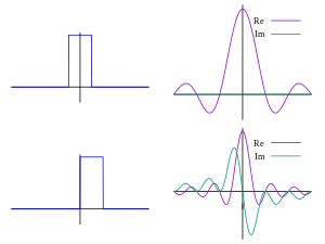
The rectangular function is Lebesgue integrable.
The sinc function, which is the Fourier transform of the rectangular function, is bounded and continuous, but not Lebesgue integrable.
The Fourier transform may be defined in some cases for non-integrable functions, but the Fourier transforms of integrable functions have several strong properties.
The Fourier transform f̂ of any integrable function f is uniformly continuous and[14]
- ‖f^‖∞≤‖f‖1{displaystyle left|{hat {f}}right|_{infty }leq left|fright|_{1}}

By the Riemann–Lebesgue lemma,[15]
- f^(ξ)→0 as |ξ|→∞.{displaystyle {hat {f}}(xi )to 0{text{ as }}|xi |to infty .}

However, f^{displaystyle {hat {f}}}
It is not generally possible to write the inverse transform as a Lebesgue integral. However, when both f and f^{displaystyle {hat {f}}}
- f(x)=∫−∞∞f^(ξ)e2iπxξdξ{displaystyle f(x)=int _{-infty }^{infty }{hat {f}}(xi )e^{2ipi xxi },dxi }

holds almost everywhere. That is, the Fourier transform is injective on L1(ℝ). (But if f is continuous, then equality holds for every x.)
Plancherel theorem and Parseval's theorem
Let f (x) and g(x) be integrable, and let f̂ (ξ) and ĝ(ξ) be their Fourier transforms. If f (x) and g(x) are also square-integrable, then we have the Parseval formula:[16]
- ∫−∞∞f(x)g(x)¯dx=∫−∞∞f^(ξ)g^(ξ)¯dξ,{displaystyle int _{-infty }^{infty }f(x){overline {g(x)}},dx=int _{-infty }^{infty }{hat {f}}(xi ){overline {{hat {g}}(xi )}},dxi ,}

where the bar denotes complex conjugation.
The Plancherel theorem, which follows from the above, states that[17]
- ∫−∞∞|f(x)|2dx=∫−∞∞|f^(ξ)|2dξ.{displaystyle int _{-infty }^{infty }left|f(x)right|^{2},dx=int _{-infty }^{infty }left|{hat {f}}(xi )right|^{2},dxi .}

Plancherel's theorem makes it possible to extend the Fourier transform, by a continuity argument, to a unitary operator on L2(ℝ). On L1(ℝ) ∩ L2(ℝ), this extension agrees with original Fourier transform defined on L1(ℝ), thus enlarging the domain of the Fourier transform to L1(ℝ) + L2(ℝ) (and consequently to Lp(ℝ) for 1 ≤ p ≤ 2). Plancherel's theorem has the interpretation in the sciences that the Fourier transform preserves the energy of the original quantity. The terminology of these formulas is not quite standardised. Parseval's theorem was proved only for Fourier series, and was first proved by Lyapunov. But Parseval's formula makes sense for the Fourier transform as well, and so even though in the context of the Fourier transform it was proved by Plancherel, it is still often referred to as Parseval's formula, or Parseval's relation, or even Parseval's theorem.
See Pontryagin duality for a general formulation of this concept in the context of locally compact abelian groups.
Poisson summation formula
The Poisson summation formula (PSF) is an equation that relates the Fourier series coefficients of the periodic summation of a function to values of the function's continuous Fourier transform. The Poisson summation formula says that for sufficiently regular functions f,
- ∑nf^(n)=∑nf(n).{displaystyle sum _{n}{hat {f}}(n)=sum _{n}f(n).}

It has a variety of useful forms that are derived from the basic one by application of the Fourier transform's scaling and time-shifting properties. The formula has applications in engineering, physics, and number theory. The frequency-domain dual of the standard Poisson summation formula is also called the discrete-time Fourier transform.
Poisson summation is generally associated with the physics of periodic media, such as heat conduction on a circle. The fundamental solution of the heat equation on a circle is called a theta function. It is used in number theory to prove the transformation properties of theta functions, which turn out to be a type of modular form, and it is connected more generally to the theory of automorphic forms where it appears on one side of the Selberg trace formula.
Differentiation
Suppose f (x) is an absolutely continuous differentiable function, and both f and its derivative f ′ are integrable. Then the Fourier transform of the derivative is given by
- f′^(ξ)=2πiξf^(ξ).{displaystyle {widehat {f';}}(xi )=2pi ixi {hat {f}}(xi ).}

More generally, the Fourier transformation of the nth derivative f(n) is given by
- f(n)^(ξ)=(2πiξ)nf^(ξ).{displaystyle {widehat {f^{(n)}}}(xi )=(2pi ixi )^{n}{hat {f}}(xi ).}

By applying the Fourier transform and using these formulas, some ordinary differential equations can be transformed into algebraic equations, which are much easier to solve. These formulas also give rise to the rule of thumb "f (x) is smooth if and only if f̂ (ξ) quickly falls to 0 for |ξ| → ∞." By using the analogous rules for the inverse Fourier transform, one can also say "f (x) quickly falls to 0 for |x| → ∞ if and only if f̂ (ξ) is smooth."
Convolution theorem
The Fourier transform translates between convolution and multiplication of functions. If f (x) and g(x) are integrable functions with Fourier transforms f̂ (ξ) and ĝ(ξ) respectively, then the Fourier transform of the convolution is given by the product of the Fourier transforms f̂ (ξ) and ĝ(ξ) (under other conventions for the definition of the Fourier transform a constant factor may appear).
This means that if:
- h(x)=(f∗g)(x)=∫−∞∞f(y)g(x−y)dy,{displaystyle h(x)=(f*g)(x)=int _{-infty }^{infty }f(y)g(x-y),dy,}

where ∗ denotes the convolution operation, then:
- h^(ξ)=f^(ξ)⋅g^(ξ).{displaystyle {hat {h}}(xi )={hat {f}}(xi )cdot {hat {g}}(xi ).}

In linear time invariant (LTI) system theory, it is common to interpret g(x) as the impulse response of an LTI system with input f (x) and output h(x), since substituting the unit impulse for f (x) yields h(x) = g(x). In this case, ĝ(ξ) represents the frequency response of the system.
Conversely, if f (x) can be decomposed as the product of two square integrable functions p(x) and q(x), then the Fourier transform of f (x) is given by the convolution of the respective Fourier transforms p̂(ξ) and q̂(ξ).
Cross-correlation theorem
In an analogous manner, it can be shown that if h(x) is the cross-correlation of f (x) and g(x):
- h(x)=(f⋆g)(x)=∫−∞∞f(y)¯g(x+y)dy{displaystyle h(x)=(fstar g)(x)=int _{-infty }^{infty }{overline {f(y)}}g(x+y),dy}

then the Fourier transform of h(x) is:
- h^(ξ)=f^(ξ)¯⋅g^(ξ).{displaystyle {hat {h}}(xi )={overline {{hat {f}}(xi )}}cdot {hat {g}}(xi ).}

As a special case, the autocorrelation of function f (x) is:
- h(x)=(f⋆f)(x)=∫−∞∞f(y)¯f(x+y)dy{displaystyle h(x)=(fstar f)(x)=int _{-infty }^{infty }{overline {f(y)}}f(x+y),dy}

for which
- h^(ξ)=f^(ξ)¯f^(ξ)=|f^(ξ)|2.{displaystyle {hat {h}}(xi )={overline {{hat {f}}(xi )}}{hat {f}}(xi )=left|{hat {f}}(xi )right|^{2}.}

Eigenfunctions
One important choice of an orthonormal basis for L2(ℝ) is given by the Hermite functions
- ψn(x)=24n!e−πx2Hen(2xπ),{displaystyle psi _{n}(x)={frac {sqrt[{4}]{2}}{sqrt {n!}}}e^{-pi x^{2}}mathrm {He} _{n}left(2x{sqrt {pi }}right),}
![{displaystyle psi _{n}(x)={frac {sqrt[{4}]{2}}{sqrt {n!}}}e^{-pi x^{2}}mathrm {He} _{n}left(2x{sqrt {pi }}right),}](https://wikimedia.org/api/rest_v1/media/math/render/svg/a9121f54a3fdbb0eedecf2aef5a379bdfae414b7)
where Hen(x) are the "probabilist's" Hermite polynomials, defined as
- Hen(x)=(−1)nex22(ddx)ne−x22{displaystyle mathrm {He} _{n}(x)=(-1)^{n}e^{frac {x^{2}}{2}}left({frac {d}{dx}}right)^{n}e^{-{frac {x^{2}}{2}}}}

Under this convention for the Fourier transform, we have that
ψ^n(ξ)=(−i)nψn(ξ){displaystyle {hat {psi }}_{n}(xi )=(-i)^{n}psi _{n}(xi )}.
In other words, the Hermite functions form a complete orthonormal system of eigenfunctions for the Fourier transform on L2(ℝ).[13] However, this choice of eigenfunctions is not unique. There are only four different eigenvalues of the Fourier transform (±1 and ±i) and any linear combination of eigenfunctions with the same eigenvalue gives another eigenfunction. As a consequence of this, it is possible to decompose L2(ℝ) as a direct sum of four spaces H0, H1, H2, and H3 where the Fourier transform acts on Hek simply by multiplication by ik.
Since the complete set of Hermite functions provides a resolution of the identity, the Fourier transform can be represented by such a sum of terms weighted by the above eigenvalues, and these sums can be explicitly summed. This approach to define the Fourier transform was first done by Norbert Wiener.[18] Among other properties, Hermite functions decrease exponentially fast in both frequency and time domains, and they are thus used to define a generalization of the Fourier transform, namely the fractional Fourier transform used in time-frequency analysis.[19] In physics, this transform was introduced by Edward Condon.[20]
Connection with the Heisenberg group
The Heisenberg group is a certain group of unitary operators on the Hilbert space L2(ℝ) of square integrable complex valued functions f on the real line, generated by the translations (Ty f )(x) = f (x + y) and multiplication by e2πixξ, (Mξ f )(x) = e2πixξf (x). These operators do not commute, as their (group) commutator is
- (Mξ−1Ty−1MξTyf)(x)=e2πiyξf(x){displaystyle left(M_{xi }^{-1}T_{y}^{-1}M_{xi }T_{y}fright)(x)=e^{2pi iyxi }f(x)}

which is multiplication by the constant (independent of x) e2πiyξ ∈ U(1) (the circle group of unit modulus complex numbers). As an abstract group, the Heisenberg group is the three-dimensional Lie group of triples (x, ξ, z) ∈ ℝ2 × U(1), with the group law
- (x1,ξ1,t1)⋅(x2,ξ2,t2)=(x1+x2,ξ1+ξ2,t1t2e2πi(x1ξ1+x2ξ2+x1ξ2)).{displaystyle left(x_{1},xi _{1},t_{1}right)cdot left(x_{2},xi _{2},t_{2}right)=left(x_{1}+x_{2},xi _{1}+xi _{2},t_{1}t_{2}e^{2pi ileft(x_{1}xi _{1}+x_{2}xi _{2}+x_{1}xi _{2}right)}right).}

Denote the Heisenberg group by H1. The above procedure describes not only the group structure, but also a standard unitary representation of H1 on a Hilbert space, which we denote by ρ : H1 → B(L2(ℝ)). Define the linear automorphism of ℝ2 by
- J(xξ)=(−ξx){displaystyle J{begin{pmatrix}x\xi end{pmatrix}}={begin{pmatrix}-xi \xend{pmatrix}}}

so that J2 = −I. This J can be extended to a unique automorphism of H1:
- j(x,ξ,t)=(−ξ,x,te−2πixξ).{displaystyle jleft(x,xi ,tright)=left(-xi ,x,te^{-2pi ixxi }right).}

According to the Stone–von Neumann theorem, the unitary representations ρ and ρ ∘ j are unitarily equivalent, so there is a unique intertwiner W ∈ U(L2(ℝ)) such that
- ρ∘j=WρW∗.{displaystyle rho circ j=Wrho W^{*}.}

This operator W is the Fourier transform.
Many of the standard properties of the Fourier transform are immediate consequences of this more general framework.[21] For example, the square of the Fourier transform, W2, is an intertwiner associated with J2 = −I, and so we have (W2f )(x) = f (−x) is the reflection of the original function f.
Complex domain
The integral for the Fourier transform
- f^(ξ)=∫−∞∞e−2πiξtf(t)dt{displaystyle {hat {f}}(xi )=int _{-infty }^{infty }e^{-2pi ixi t}f(t),dt}

can be studied for complex values of its argument ξ. Depending on the properties of f, this might not converge off the real axis at all, or it might converge to a complex analytic function for all values of ξ = σ + iτ, or something in between.[22]
The Paley–Wiener theorem says that f is smooth (i.e., n-times differentiable for all positive integers n) and compactly supported if and only if f̂ (σ + iτ) is a holomorphic function for which there exists a constant a > 0 such that for any integer n ≥ 0,
- |ξnf^(ξ)|≤Cea|τ|{displaystyle leftvert xi ^{n}{hat {f}}(xi )rightvert leq Ce^{avert tau vert }}

for some constant C. (In this case, f is supported on [−a, a].) This can be expressed by saying that f̂ is an entire function which is rapidly decreasing in σ (for fixed τ) and of exponential growth in τ (uniformly in σ).[23]
(If f is not smooth, but only L2, the statement still holds provided n = 0.[24]) The space of such functions of a complex variable is called the Paley—Wiener space. This theorem has been generalised to semisimple Lie groups.[25]
If f is supported on the half-line t ≥ 0, then f is said to be "causal" because the impulse response function of a physically realisable filter must have this property, as no effect can precede its cause. Paley and Wiener showed that then f̂ extends to a holomorphic function on the complex lower half-plane τ < 0 which tends to zero as τ goes to infinity.[26] The converse is false and it is not known how to characterise the Fourier transform of a causal function.[27]
Laplace transform
The Fourier transform f̂ (ξ) is related to the Laplace transform F(s), which is also used for the solution of differential equations and the analysis of filters.
It may happen that a function f for which the Fourier integral does not converge on the real axis at all, nevertheless has a complex Fourier transform defined in some region of the complex plane.
For example, if f (t) is of exponential growth, i.e.,
- |f(t)|<Cea|t|{displaystyle vert f(t)vert <Ce^{avert tvert }}

for some constants C, a ≥ 0, then[28]
- f^(iτ)=∫−∞∞e2πτtf(t)dt,{displaystyle {hat {f}}(itau )=int _{-infty }^{infty }e^{2pi tau t}f(t),dt,}

convergent for all 2πτ < −a, is the two-sided Laplace transform of f.
The more usual version ("one-sided") of the Laplace transform is
- F(s)=∫0∞f(t)e−stdt.{displaystyle F(s)=int _{0}^{infty }f(t)e^{-st},dt.}

If f is also causal, then
- f^(iτ)=F(−2πτ).{displaystyle {hat {f}}(itau )=F(-2pi tau ).}

Thus, extending the Fourier transform to the complex domain means it includes the Laplace transform as a special case—the case of causal functions—but with the change of variable s = 2πiξ.
Inversion
If f̂ is complex analytic for a ≤ τ ≤ b, then
- ∫−∞∞f^(σ+ia)e2πiξtdσ=∫−∞∞f^(σ+ib)e2πiξtdσ{displaystyle int _{-infty }^{infty }{hat {f}}(sigma +ia)e^{2pi ixi t},dsigma =int _{-infty }^{infty }{hat {f}}(sigma +ib)e^{2pi ixi t},dsigma }

by Cauchy's integral theorem. Therefore, the Fourier inversion formula can use integration along different lines, parallel to the real axis.[29]
Theorem: If f (t) = 0 for t < 0, and |f (t)| < Cea|t| for some constants C, a > 0, then
- f(t)=∫−∞∞f^(σ+iτ)e2πiξtdσ,{displaystyle f(t)=int _{-infty }^{infty }{hat {f}}(sigma +itau )e^{2pi ixi t},dsigma ,}

for any τ < −a/2π.
This theorem implies the Mellin inversion formula for the Laplace transformation,[28]
- f(t)=12πi∫b−i∞b+i∞F(s)estds{displaystyle f(t)={frac {1}{2pi i}}int _{b-iinfty }^{b+iinfty }F(s)e^{st},ds}

for any b > a, where F(s) is the Laplace transform of f (t).
The hypotheses can be weakened, as in the results of Carleman and Hunt, to f (t) e−at being L1, provided that f is of bounded variation in a closed neighborhood of t (cf. Dirichlet-Dini theorem), the value of f at t is taken to be the arithmetic mean of the left and right limits, and provided that the integrals are taken in the sense of Cauchy principal values.[30]
L2 versions of these inversion formulas are also available.[31]
Fourier transform on Euclidean space
The Fourier transform can be defined in any arbitrary number of dimensions n. As with the one-dimensional case, there are many conventions. For an integrable function f (x), this article takes the definition:
- f^(ξ)=F(f)(ξ)=∫Rnf(x)e−2πix⋅ξdx{displaystyle {hat {f}}({boldsymbol {xi }})={mathcal {F}}(f)({boldsymbol {xi }})=int _{mathbb {R} ^{n}}f(mathbf {x} )e^{-2pi imathbf {x} cdot {boldsymbol {xi }}},dmathbf {x} }

where x and ξ are n-dimensional vectors, and x · ξ is the dot product of the vectors. The dot product is sometimes written as ⟨x, ξ⟩.
All of the basic properties listed above hold for the n-dimensional Fourier transform, as do Plancherel's and Parseval's theorem. When the function is integrable, the Fourier transform is still uniformly continuous and the Riemann–Lebesgue lemma holds.[15]
Uncertainty principle
Generally speaking, the more concentrated f (x) is, the more spread out its Fourier transform f̂ (ξ) must be. In particular, the scaling property of the Fourier transform may be seen as saying: if we squeeze a function in x, its Fourier transform stretches out in ξ. It is not possible to arbitrarily concentrate both a function and its Fourier transform.
The trade-off between the compaction of a function and its Fourier transform can be formalized in the form of an uncertainty principle by viewing a function and its Fourier transform as conjugate variables with respect to the symplectic form on the time–frequency domain: from the point of view of the linear canonical transformation, the Fourier transform is rotation by 90° in the time–frequency domain, and preserves the symplectic form.
Suppose f (x) is an integrable and square-integrable function. Without loss of generality, assume that f (x) is normalized:
- ∫−∞∞|f(x)|2dx=1.{displaystyle int _{-infty }^{infty }|f(x)|^{2},dx=1.}

It follows from the Plancherel theorem that f̂ (ξ) is also normalized.
The spread around x = 0 may be measured by the dispersion about zero[32] defined by
- D0(f)=∫−∞∞x2|f(x)|2dx.{displaystyle D_{0}(f)=int _{-infty }^{infty }x^{2}|f(x)|^{2},dx.}

In probability terms, this is the second moment of |f (x)|2 about zero.
The Uncertainty principle states that, if f (x) is absolutely continuous and the functions x·f (x) and f ′(x) are square integrable, then[13]
D0(f)D0(f^)≥116π2{displaystyle D_{0}(f)D_{0}left({hat {f}}right)geq {frac {1}{16pi ^{2}}}}.
The equality is attained only in the case
- f(x)=C1e−πx2σ2∴f^(ξ)=σC1e−πσ2ξ2{displaystyle {begin{aligned}f(x)&=C_{1},e^{-pi {frac {x^{2}}{sigma ^{2}}}}\therefore {hat {f}}(xi )&=sigma C_{1},e^{-pi sigma ^{2}xi ^{2}}end{aligned}}}

where σ > 0 is arbitrary and C1 = 4√2/√σ so that f is L2-normalized.[13] In other words, where f is a (normalized) Gaussian function with variance σ2, centered at zero, and its Fourier transform is a Gaussian function with variance σ−2.
In fact, this inequality implies that:
- (∫−∞∞(x−x0)2|f(x)|2dx)(∫−∞∞(ξ−ξ0)2|f^(ξ)|2dξ)≥116π2{displaystyle left(int _{-infty }^{infty }(x-x_{0})^{2}|f(x)|^{2},dxright)left(int _{-infty }^{infty }(xi -xi _{0})^{2}left|{hat {f}}(xi )right|^{2},dxi right)geq {frac {1}{16pi ^{2}}}}

for any x0, ξ0 ∈ ℝ.[12]
In quantum mechanics, the momentum and position wave functions are Fourier transform pairs, to within a factor of Planck's constant. With this constant properly taken into account, the inequality above becomes the statement of the Heisenberg uncertainty principle.[33]
A stronger uncertainty principle is the Hirschman uncertainty principle, which is expressed as:
- H(|f|2)+H(|f^|2)≥log(e2){displaystyle Hleft(left|fright|^{2}right)+Hleft(left|{hat {f}}right|^{2}right)geq log left({frac {e}{2}}right)}

where H(p) is the differential entropy of the probability density function p(x):
- H(p)=−∫−∞∞p(x)log(p(x))dx{displaystyle H(p)=-int _{-infty }^{infty }p(x)log {bigl (}p(x){bigr )},dx}

where the logarithms may be in any base that is consistent. The equality is attained for a Gaussian, as in the previous case.
Sine and cosine transforms
Fourier's original formulation of the transform did not use complex numbers, but rather sines and cosines. Statisticians and others still use this form. An absolutely integrable function f for which Fourier inversion holds good can be expanded in terms of genuine frequencies (avoiding negative frequencies, which are sometimes considered hard to interpret physically[34]) λ by
- f(t)=∫0∞(a(λ)cos(2πλt)+b(λ)sin(2πλt))dλ.{displaystyle f(t)=int _{0}^{infty }{bigl (}a(lambda )cos(2pi lambda t)+b(lambda )sin(2pi lambda t){bigr )},dlambda .}

This is called an expansion as a trigonometric integral, or a Fourier integral expansion. The coefficient functions a and b can be found by using variants of the Fourier cosine transform and the Fourier sine transform (the normalisations are, again, not standardised):
- a(λ)=2∫−∞∞f(t)cos(2πλt)dt{displaystyle a(lambda )=2int _{-infty }^{infty }f(t)cos(2pi lambda t),dt}

and
- b(λ)=2∫−∞∞f(t)sin(2πλt)dt.{displaystyle b(lambda )=2int _{-infty }^{infty }f(t)sin(2pi lambda t),dt.}

Older literature refers to the two transform functions, the Fourier cosine transform, a, and the Fourier sine transform, b.
The function f can be recovered from the sine and cosine transform using
- f(t)=2∫0∞∫−∞∞f(τ)cos(2πλ(τ−t))dτdλ.{displaystyle f(t)=2int _{0}^{infty }int _{-infty }^{infty }f(tau )cos {bigl (}2pi lambda (tau -t){bigr )},dtau ,dlambda .}

together with trigonometric identities. This is referred to as Fourier's integral formula.[28][35][36][37]
Spherical harmonics
Let the set of homogeneous harmonic polynomials of degree k on ℝn be denoted by Ak. The set Ak consists of the solid spherical harmonics of degree k. The solid spherical harmonics play a similar role in higher dimensions to the Hermite polynomials in dimension one. Specifically, if f (x) = e−π|x|2P(x) for some P(x) in Ak, then f̂ (ξ) = i−k f (ξ). Let the set Hk be the closure in L2(ℝn) of linear combinations of functions of the form f (|x|)P(x) where P(x) is in Ak. The space L2(ℝn) is then a direct sum of the spaces Hk and the Fourier transform maps each space Hk to itself and is possible to characterize the action of the Fourier transform on each space Hk.[15]
Let f (x) = f0(|x|)P(x) (with P(x) in Ak), then
- f^(ξ)=F0(|ξ|)P(ξ){displaystyle {hat {f}}(xi )=F_{0}(|xi |)P(xi )}

where
- F0(r)=2πi−kr−n+2k−22∫0∞f0(s)Jn+2k−22(2πrs)sn+2k2ds.{displaystyle F_{0}(r)=2pi i^{-k}r^{-{frac {n+2k-2}{2}}}int _{0}^{infty }f_{0}(s)J_{frac {n+2k-2}{2}}(2pi rs)s^{frac {n+2k}{2}},ds.}

Here Jn + 2k − 2/2 denotes the Bessel function of the first kind with order n + 2k − 2/2. When k = 0 this gives a useful formula for the Fourier transform of a radial function.[38] Note that this is essentially the Hankel transform. Moreover, there is a simple recursion relating the cases n + 2 and n[39] allowing to compute, e.g., the three-dimensional Fourier transform of a radial function from the one-dimensional one.
Restriction problems
In higher dimensions it becomes interesting to study restriction problems for the Fourier transform. The Fourier transform of an integrable function is continuous and the restriction of this function to any set is defined. But for a square-integrable function the Fourier transform could be a general class of square integrable functions. As such, the restriction of the Fourier transform of an L2(ℝn) function cannot be defined on sets of measure 0. It is still an active area of study to understand restriction problems in Lp for 1 < p < 2. Surprisingly, it is possible in some cases to define the restriction of a Fourier transform to a set S, provided S has non-zero curvature. The case when S is the unit sphere in ℝn is of particular interest. In this case the Tomas–Stein restriction theorem states that the restriction of the Fourier transform to the unit sphere in ℝn is a bounded operator on Lp provided 1 ≤ p ≤ 2n + 2/n + 3.
One notable difference between the Fourier transform in 1 dimension versus higher dimensions concerns the partial sum operator. Consider an increasing collection of measurable sets ER indexed by R ∈ (0,∞): such as balls of radius R centered at the origin, or cubes of side 2R. For a given integrable function f, consider the function fR defined by:
- fR(x)=∫ERf^(ξ)e2πix⋅ξdξ,x∈Rn.{displaystyle f_{R}(x)=int _{E_{R}}{hat {f}}(xi )e^{2pi ixcdot xi },dxi ,quad xin mathbb {R} ^{n}.}

Suppose in addition that f ∈ Lp(ℝn). For n = 1 and 1 < p < ∞, if one takes ER = (−R, R), then fR converges to f in Lp as R tends to infinity, by the boundedness of the Hilbert transform. Naively one may hope the same holds true for n > 1. In the case that ER is taken to be a cube with side length R, then convergence still holds. Another natural candidate is the Euclidean ball ER = {ξ : |ξ| < R}. In order for this partial sum operator to converge, it is necessary that the multiplier for the unit ball be bounded in Lp(ℝn). For n ≥ 2 it is a celebrated theorem of Charles Fefferman that the multiplier for the unit ball is never bounded unless p = 2.[18] In fact, when p ≠ 2, this shows that not only may fR fail to converge to f in Lp, but for some functions f ∈ Lp(ℝn), fR is not even an element of Lp.
Fourier transform on function spaces
On Lp spaces
On L1
The definition of the Fourier transform by the integral formula
- f^(ξ)=∫Rnf(x)e−2πiξ⋅xdx{displaystyle {hat {f}}(xi )=int _{mathbb {R} ^{n}}f(x)e^{-2pi ixi cdot x},dx}

is valid for Lebesgue integrable functions f; that is, f ∈ L1(ℝn).
The Fourier transform F : L1(ℝn) → L∞(ℝn) is a bounded operator. This follows from the observation that
- |f^(ξ)|≤∫Rn|f(x)|dx,{displaystyle leftvert {hat {f}}(xi )rightvert leq int _{mathbb {R} ^{n}}vert f(x)vert ,dx,}

which shows that its operator norm is bounded by 1. Indeed, it equals 1, which can be seen, for example, from the transform of the rect function. The image of L1 is a subset of the space C0(ℝn) of continuous functions that tend to zero at infinity (the Riemann–Lebesgue lemma), although it is not the entire space. Indeed, there is no simple characterization of the image.
On L2
Since compactly supported smooth functions are integrable and dense in L2(ℝn), the Plancherel theorem allows us to extend the definition of the Fourier transform to general functions in L2(ℝn) by continuity arguments. The Fourier transform in L2(ℝn) is no longer given by an ordinary Lebesgue integral, although it can be computed by an improper integral, here meaning that for an L2 function f,
- f^(ξ)=limR→∞∫|x|≤Rf(x)e−2πix⋅ξdx{displaystyle {hat {f}}(xi )=lim _{Rto infty }int _{|x|leq R}f(x)e^{-2pi ixcdot xi },dx}

where the limit is taken in the L2 sense. (More generally, you can take a sequence of functions that are in the intersection of L1 and L2 and that converges to f in the L2-norm, and define the Fourier transform of f as the L2 -limit of the Fourier transforms of these functions.[40])
Many of the properties of the Fourier transform in L1 carry over to L2, by a suitable limiting argument.
Furthermore, F : L2(ℝn) → L2(ℝn) is a unitary operator.[41] For an operator to be unitary it is sufficient to show that it is bijective and preserves the inner product, so in this case these follow from the Fourier inversion theorem combined with the fact that for any f, g ∈ L2(ℝn) we have
- ∫Rnf(x)Fg(x)dx=∫RnFf(x)g(x)dx.{displaystyle int _{mathbb {R} ^{n}}f(x){mathcal {F}}g(x),dx=int _{mathbb {R} ^{n}}{mathcal {F}}f(x)g(x),dx.}

In particular, the image of L2(ℝn) is itself under the Fourier transform.
On other Lp
The definition of the Fourier transform can be extended to functions in Lp(ℝn) for 1 ≤ p ≤ 2 by decomposing such functions into a fat tail part in L2 plus a fat body part in L1. In each of these spaces, the Fourier transform of a function in Lp(ℝn) is in Lq(ℝn), where q = p/p − 1 is the Hölder conjugate of p (by the Hausdorff–Young inequality). However, except for p = 2, the image is not easily characterized. Further extensions become more technical. The Fourier transform of functions in Lp for the range 2 < p < ∞ requires the study of distributions.[14] In fact, it can be shown that there are functions in Lp with p > 2 so that the Fourier transform is not defined as a function.[15]
Tempered distributions
One might consider enlarging the domain of the Fourier transform from L1 + L2 by considering generalized functions, or distributions. A distribution on ℝn is a continuous linear functional on the space Cc(ℝn) of compactly supported smooth functions, equipped with a suitable topology. The strategy is then to consider the action of the Fourier transform on Cc(ℝn) and pass to distributions by duality. The obstruction to doing this is that the Fourier transform does not map Cc(ℝn) to Cc(ℝn). In fact the Fourier transform of an element in Cc(ℝn) can not vanish on an open set; see the above discussion on the uncertainty principle. The right space here is the slightly larger space of Schwartz functions. The Fourier transform is an automorphism on the Schwartz space, as a topological vector space, and thus induces an automorphism on its dual, the space of tempered distributions.[15] The tempered distributions include all the integrable functions mentioned above, as well as well-behaved functions of polynomial growth and distributions of compact support.
For the definition of the Fourier transform of a tempered distribution, let f and g be integrable functions, and let f̂ and ĝ be their Fourier transforms respectively. Then the Fourier transform obeys the following multiplication formula,[15]
- ∫Rnf^(x)g(x)dx=∫Rnf(x)g^(x)dx.{displaystyle int _{mathbb {R} ^{n}}{hat {f}}(x)g(x),dx=int _{mathbb {R} ^{n}}f(x){hat {g}}(x),dx.}

Every integrable function f defines (induces) a distribution Tf by the relation
- Tf(φ)=∫Rnf(x)φ(x)dx{displaystyle T_{f}(varphi )=int _{mathbb {R} ^{n}}f(x)varphi (x),dx}

for all Schwartz functions φ. So it makes sense to define Fourier transform T̂f of Tf by
- T^f(φ)=Tf(φ^){displaystyle {hat {T}}_{f}(varphi )=T_{f}left({hat {varphi }}right)}

for all Schwartz functions φ. Extending this to all tempered distributions T gives the general definition of the Fourier transform.
Distributions can be differentiated and the above-mentioned compatibility of the Fourier transform with differentiation and convolution remains true for tempered distributions.
Generalizations
Fourier–Stieltjes transform
The Fourier transform of a finite Borel measure μ on ℝn is given by:[42]
- μ^(ξ)=∫Rne−2πix⋅ξdμ.{displaystyle {hat {mu }}(xi )=int _{mathbb {R} ^{n}}e^{-2pi ixcdot xi },dmu .}

This transform continues to enjoy many of the properties of the Fourier transform of integrable functions. One notable difference is that the Riemann–Lebesgue lemma fails for measures.[14] In the case that dμ = f (x) dx, then the formula above reduces to the usual definition for the Fourier transform of f. In the case that μ is the probability distribution associated to a random variable X, the Fourier–Stieltjes transform is closely related to the characteristic function, but the typical conventions in probability theory take eixξ instead of e−2πixξ.[13] In the case when the distribution has a probability density function this definition reduces to the Fourier transform applied to the probability density function, again with a different choice of constants.
The Fourier transform may be used to give a characterization of measures. Bochner's theorem characterizes which functions may arise as the Fourier–Stieltjes transform of a positive measure on the circle.[14]
Furthermore, the Dirac delta function, although not a function, is a finite Borel measure. Its Fourier transform is a constant function (whose specific value depends upon the form of the Fourier transform used).
Locally compact abelian groups
The Fourier transform may be generalized to any locally compact abelian group. A locally compact abelian group is an abelian group that is at the same time a locally compact Hausdorff topological space so that the group operation is continuous. If G is a locally compact abelian group, it has a translation invariant measure μ, called Haar measure. For a locally compact abelian group G, the set of irreducible, i.e. one-dimensional, unitary representations are called its characters. With its natural group structure and the topology of pointwise convergence, the set of characters Ĝ is itself a locally compact abelian group, called the Pontryagin dual of G. For a function f in L1(G), its Fourier transform is defined by[14]
- f^(ξ)=∫Gξ(x)f(x)dμfor any ξ∈G^.{displaystyle {hat {f}}(xi )=int _{G}xi (x)f(x),dmu qquad {text{for any }}xi in {hat {G}}.}

The Riemann–Lebesgue lemma holds in this case; f̂ (ξ) is a function vanishing at infinity on Ĝ.
Gelfand transform
The Fourier transform is also a special case of Gelfand transform. In this particular context, it is closely related to the Pontryagin duality map defined above.
Given an abelian locally compact Hausdorff topological group G, as before we consider space L1(G), defined using a Haar measure. With convolution as multiplication, L1(G) is an abelian Banach algebra. It also has an involution * given by
- f∗(g)=f(g−1)¯.{displaystyle f^{*}(g)={overline {fleft(g^{-1}right)}}.}

Taking the completion with respect to the largest possibly C*-norm gives its enveloping C*-algebra, called the group C*-algebra C*(G) of G. (Any C*-norm on L1(G) is bounded by the L1 norm, therefore their supremum exists.)
Given any abelian C*-algebra A, the Gelfand transform gives an isomorphism between A and C0(A^), where A^ is the multiplicative linear functionals, i.e. one-dimensional representations, on A with the weak-* topology. The map is simply given by
- a↦(φ↦φ(a)){displaystyle amapsto {bigl (}varphi mapsto varphi (a){bigr )}}

It turns out that the multiplicative linear functionals of C*(G), after suitable identification, are exactly the characters of G, and the Gelfand transform, when restricted to the dense subset L1(G) is the Fourier–Pontryagin transform.
Compact non-abelian groups
The Fourier transform can also be defined for functions on a non-abelian group, provided that the group is compact. Removing the assumption that the underlying group is abelian, irreducible unitary representations need not always be one-dimensional. This means the Fourier transform on a non-abelian group takes values as Hilbert space operators.[43] The Fourier transform on compact groups is a major tool in representation theory[44] and non-commutative harmonic analysis.
Let G be a compact Hausdorff topological group. Let Σ denote the collection of all isomorphism classes of finite-dimensional irreducible unitary representations, along with a definite choice of representation U(σ) on the Hilbert space Hσ of finite dimension dσ for each σ ∈ Σ. If μ is a finite Borel measure on G, then the Fourier–Stieltjes transform of μ is the operator on Hσ defined by
- ⟨μ^ξ,η⟩Hσ=∫G⟨U¯g(σ)ξ,η⟩dμ(g){displaystyle leftlangle {hat {mu }}xi ,eta rightrangle _{H_{sigma }}=int _{G}leftlangle {overline {U}}_{g}^{(sigma )}xi ,eta rightrangle ,dmu (g)}

where U(σ) is the complex-conjugate representation of U(σ) acting on Hσ. If μ is absolutely continuous with respect to the left-invariant probability measure λ on G, represented as
- dμ=fdλ{displaystyle dmu =f,dlambda }

for some f ∈ L1(λ), one identifies the Fourier transform of f with the Fourier–Stieltjes transform of μ.
The mapping
- μ↦μ^{displaystyle mu mapsto {hat {mu }}}

defines an isomorphism between the Banach space M(G) of finite Borel measures (see rca space) and a closed subspace of the Banach space C∞(Σ) consisting of all sequences E = (Eσ) indexed by Σ of (bounded) linear operators Eσ : Hσ → Hσ for which the norm
- ‖E‖=supσ∈Σ‖Eσ‖{displaystyle |E|=sup _{sigma in Sigma }left|E_{sigma }right|}

is finite. The "convolution theorem" asserts that, furthermore, this isomorphism of Banach spaces is in fact an isometric isomorphism of C* algebras into a subspace of C∞(Σ). Multiplication on M(G) is given by convolution of measures and the involution * defined by
- f∗(g)=f(g−1)¯,{displaystyle f^{*}(g)={overline {fleft(g^{-1}right)}},}

and C∞(Σ) has a natural C*-algebra structure as Hilbert space operators.
The Peter–Weyl theorem holds, and a version of the Fourier inversion formula (Plancherel's theorem) follows: if f ∈ L2(G), then
- f(g)=∑σ∈Σdσtr(f^(σ)Ug(σ)){displaystyle f(g)=sum _{sigma in Sigma }d_{sigma }operatorname {tr} left({hat {f}}(sigma )U_{g}^{(sigma )}right)}

where the summation is understood as convergent in the L2 sense.
The generalization of the Fourier transform to the noncommutative situation has also in part contributed to the development of noncommutative geometry.[citation needed] In this context, a categorical generalization of the Fourier transform to noncommutative groups is Tannaka–Krein duality, which replaces the group of characters with the category of representations. However, this loses the connection with harmonic functions.
Alternatives
In signal processing terms, a function (of time) is a representation of a signal with perfect time resolution, but no frequency information, while the Fourier transform has perfect frequency resolution, but no time information: the magnitude of the Fourier transform at a point is how much frequency content there is, but location is only given by phase (argument of the Fourier transform at a point), and standing waves are not localized in time – a sine wave continues out to infinity, without decaying. This limits the usefulness of the Fourier transform for analyzing signals that are localized in time, notably transients, or any signal of finite extent.
As alternatives to the Fourier transform, in time-frequency analysis, one uses time-frequency transforms or time-frequency distributions to represent signals in a form that has some time information and some frequency information – by the uncertainty principle, there is a trade-off between these. These can be generalizations of the Fourier transform, such as the short-time Fourier transform or fractional Fourier transform, or other functions to represent signals, as in wavelet transforms and chirplet transforms, with the wavelet analog of the (continuous) Fourier transform being the continuous wavelet transform.[19]
Applications
Some problems, such as certain differential equations, become easier to solve when the Fourier transform is applied. In that case the solution to the original problem is recovered using the inverse Fourier transform.
Analysis of differential equations
Perhaps the most important use of the Fourier transformation is to solve partial differential equations.
Many of the equations of the mathematical physics of the nineteenth century can be treated this way. Fourier studied the heat equation, which in one dimension and in dimensionless units is
- ∂2y(x,t)∂2x=∂y(x,t)∂t.{displaystyle {frac {partial ^{2}y(x,t)}{partial ^{2}x}}={frac {partial y(x,t)}{partial t}}.}

The example we will give, a slightly more difficult one, is the wave equation in one dimension,
- ∂2y(x,t)∂2x=∂2y(x,t)∂2t.{displaystyle {frac {partial ^{2}y(x,t)}{partial ^{2}x}}={frac {partial ^{2}y(x,t)}{partial ^{2}t}}.}

As usual, the problem is not to find a solution: there are infinitely many. The problem is that of the so-called "boundary problem": find a solution which satisfies the "boundary conditions"
- y(x,0)=f(x),∂y(x,0)∂t=g(x).{displaystyle y(x,0)=f(x),qquad {frac {partial y(x,0)}{partial t}}=g(x).}

Here, f and g are given functions. For the heat equation, only one boundary condition can be required (usually the first one). But for the wave equation, there are still infinitely many solutions y which satisfy the first boundary condition. But when one imposes both conditions, there is only one possible solution.
It is easier to find the Fourier transform ŷ of the solution than to find the solution directly. This is because the Fourier transformation takes differentiation into multiplication by the variable, and so a partial differential equation applied to the original function is transformed into multiplication by polynomial functions of the dual variables applied to the transformed function. After ŷ is determined, we can apply the inverse Fourier transformation to find y.
Fourier's method is as follows. First, note that any function of the forms
- cos(2πξ(x±t)) or sin(2πξ(x±t)){displaystyle cos {bigl (}2pi xi (xpm t){bigr )}{mbox{ or }}sin {bigl (}2pi xi (xpm t){bigr )}}

satisfies the wave equation. These are called the elementary solutions.
Second, note that therefore any integral
- y(x,t)=∫0∞a+(ξ)cos(2πξ(x+t))+a−(ξ)cos(2πξ(x−t))+b+(ξ)sin(2πξ(x+t))+b−(ξ)sin(2πξ(x−t))dξ{displaystyle y(x,t)=int _{0}^{infty }a_{+}(xi )cos {bigl (}2pi xi (x+t){bigr )}+a_{-}(xi )cos {bigl (}2pi xi (x-t){bigr )}+b_{+}(xi )sin {bigl (}2pi xi (x+t){bigr )}+b_{-}(xi )sin left(2pi xi (x-t)right),dxi }

(for arbitrary a+, a−, b+, b−) satisfies the wave equation. (This integral is just a kind of continuous linear combination, and the equation is linear.)
Now this resembles the formula for the Fourier synthesis of a function. In fact, this is the real inverse Fourier transform of a± and b± in the variable x.
The third step is to examine how to find the specific unknown coefficient functions a± and b± that will lead to y satisfying the boundary conditions. We are interested in the values of these solutions at t = 0. So we will set t = 0. Assuming that the conditions needed for Fourier inversion are satisfied, we can then find the Fourier sine and cosine transforms (in the variable x) of both sides and obtain
- 2∫−∞∞y(x,0)cos(2πξx)dx=a++a−{displaystyle 2int _{-infty }^{infty }y(x,0)cos(2pi xi x),dx=a_{+}+a_{-}}

and
- 2∫−∞∞y(x,0)sin(2πξx)dx=b++b−.{displaystyle 2int _{-infty }^{infty }y(x,0)sin(2pi xi x),dx=b_{+}+b_{-}.}

Similarly, taking the derivative of y with respect to t and then applying the Fourier sine and cosine transformations yields
- 2∫−∞∞∂y(u,0)∂tsin(2πξx)dx=(2πξ)(−a++a−){displaystyle 2int _{-infty }^{infty }{frac {partial y(u,0)}{partial t}}sin(2pi xi x),dx=(2pi xi )left(-a_{+}+a_{-}right)}

and
- 2∫−∞∞∂y(u,0)∂tcos(2πξx)dx=(2πξ)(b+−b−).{displaystyle 2int _{-infty }^{infty }{frac {partial y(u,0)}{partial t}}cos(2pi xi x),dx=(2pi xi )left(b_{+}-b_{-}right).}

These are four linear equations for the four unknowns a± and b±, in terms of the Fourier sine and cosine transforms of the boundary conditions, which are easily solved by elementary algebra, provided that these transforms can be found.
In summary, we chose a set of elementary solutions, parametrised by ξ, of which the general solution would be a (continuous) linear combination in the form of an integral over the parameter ξ. But this integral was in the form of a Fourier integral. The next step was to express the boundary conditions in terms of these integrals, and set them equal to the given functions f and g. But these expressions also took the form of a Fourier integral because of the properties of the Fourier transform of a derivative. The last step was to exploit Fourier inversion by applying the Fourier transformation to both sides, thus obtaining expressions for the coefficient functions a± and b± in terms of the given boundary conditions f and g.
From a higher point of view, Fourier's procedure can be reformulated more conceptually. Since there are two variables, we will use the Fourier transformation in both x and t rather than operate as Fourier did, who only transformed in the spatial variables. Note that ŷ must be considered in the sense of a distribution since y(x, t) is not going to be L1: as a wave, it will persist through time and thus is not a transient phenomenon. But it will be bounded and so its Fourier transform can be defined as a distribution. The operational properties of the Fourier transformation that are relevant to this equation are that it takes differentiation in x to multiplication by 2πiξ and differentiation with respect to t to multiplication by 2πif where f is the frequency. Then the wave equation becomes an algebraic equation in ŷ:
- ξ2y^(ξ,f)=f2y^(ξ,f).{displaystyle xi ^{2}{hat {y}}(xi ,f)=f^{2}{hat {y}}(xi ,f).}

This is equivalent to requiring ŷ(ξ, f ) = 0 unless ξ = ±f. Right away, this explains why the choice of elementary solutions we made earlier worked so well: obviously f̂ = δ(ξ ± f ) will be solutions. Applying Fourier inversion to these delta functions, we obtain the elementary solutions we picked earlier. But from the higher point of view, one does not pick elementary solutions, but rather considers the space of all distributions which are supported on the (degenerate) conic ξ2 − f2 = 0.
We may as well consider the distributions supported on the conic that are given by distributions of one variable on the line ξ = f plus distributions on the line ξ = −f as follows: if ϕ is any test function,
- ∬y^ϕ(ξ,f)dξdf=∫s+ϕ(ξ,ξ)dξ+∫s−ϕ(ξ,−ξ)dξ,{displaystyle iint {hat {y}}phi (xi ,f),dxi ,df=int s_{+}phi (xi ,xi ),dxi +int s_{-}phi (xi ,-xi ),dxi ,}

where s+, and s−, are distributions of one variable.
Then Fourier inversion gives, for the boundary conditions, something very similar to what we had more concretely above (put ϕ(ξ, f ) = e2πi(xξ+tf ), which is clearly of polynomial growth):
- y(x,0)=∫{s+(ξ)+s−(ξ)}e2πiξx+0dξ{displaystyle y(x,0)=int {bigl {}s_{+}(xi )+s_{-}(xi ){bigr }}e^{2pi ixi x+0},dxi }

and
- ∂y(x,0)∂t=∫{s+(ξ)−s−(ξ)}2πiξe2πiξx+0dξ.{displaystyle {frac {partial y(x,0)}{partial t}}=int {bigl {}s_{+}(xi )-s_{-}(xi ){bigr }}2pi ixi e^{2pi ixi x+0},dxi .}

Now, as before, applying the one-variable Fourier transformation in the variable x to these functions of x yields two equations in the two unknown distributions s± (which can be taken to be ordinary functions if the boundary conditions are L1 or L2).
From a calculational point of view, the drawback of course is that one must first calculate the Fourier transforms of the boundary conditions, then assemble the solution from these, and then calculate an inverse Fourier transform. Closed form formulas are rare, except when there is some geometric symmetry that can be exploited, and the numerical calculations are difficult because of the oscillatory nature of the integrals, which makes convergence slow and hard to estimate. For practical calculations, other methods are often used.
The twentieth century has seen the extension of these methods to all linear partial differential equations with polynomial coefficients, and by extending the notion of Fourier transformation to include Fourier integral operators, some non-linear equations as well.
Fourier transform spectroscopy
The Fourier transform is also used in nuclear magnetic resonance (NMR) and in other kinds of spectroscopy, e.g. infrared (FTIR). In NMR an exponentially shaped free induction decay (FID) signal is acquired in the time domain and Fourier-transformed to a Lorentzian line-shape in the frequency domain. The Fourier transform is also used in magnetic resonance imaging (MRI) and mass spectrometry.
Quantum mechanics
The Fourier transform is useful in quantum mechanics in two different ways. To begin with, the basic conceptual structure of Quantum Mechanics postulates the existence of pairs of complementary variables, connected by the Heisenberg uncertainty principle. For example, in one dimension, the spatial variable q of, say, a particle, can only be measured by the quantum mechanical "position operator" at the cost of losing information about the momentum p of the particle. Therefore, the physical state of the particle can either be described by a function, called "the wave function", of q or by a function of p but not by a function of both variables. The variable p is called the conjugate variable to q. In Classical Mechanics, the physical state of a particle (existing in one dimension, for simplicity of exposition) would be given by assigning definite values to both p and q simultaneously. Thus, the set of all possible physical states is the two-dimensional real vector space with a p-axis and a q-axis called the phase space.
In contrast, quantum mechanics chooses a polarisation of this space in the sense that it picks a subspace of one-half the dimension, for example, the q-axis alone, but instead of considering only points, takes the set of all complex-valued "wave functions" on this axis. Nevertheless, choosing the p-axis is an equally valid polarisation, yielding a different representation of the set of possible physical states of the particle which is related to the first representation by the Fourier transformation
- ϕ(p)=∫ψ(q)e2πipqhdq.{displaystyle phi (p)=int psi (q)e^{2pi i{frac {pq}{h}}},dq.}

Physically realisable states are L2, and so by the Plancherel theorem, their Fourier transforms are also L2. (Note that since q is in units of distance and p is in units of momentum, the presence of Planck's constant in the exponent makes the exponent dimensionless, as it should be.)
Therefore, the Fourier transform can be used to pass from one way of representing the state of the particle, by a wave function of position, to another way of representing the state of the particle: by a wave function of momentum. Infinitely many different polarisations are possible, and all are equally valid. Being able to transform states from one representation to another is sometimes convenient.
The other use of the Fourier transform in both quantum mechanics and quantum field theory is to solve the applicable wave equation. In non-relativistic quantum mechanics, Schrödinger's equation for a time-varying wave function in one-dimension, not subject to external forces, is
- ∂2∂x2ψ(x,t)=ih2π∂∂tψ(x,t).{displaystyle {frac {partial ^{2}}{partial x^{2}}}psi (x,t)=i{frac {h}{2pi }}{frac {partial }{partial t}}psi (x,t).}

This is the same as the heat equation except for the presence of the imaginary unit i. Fourier methods can be used to solve this equation.
In the presence of a potential, given by the potential energy function V(x), the equation becomes
- ∂2∂x2ψ(x,t)+V(x)ψ(x,t)=ih2π∂∂tψ(x,t).{displaystyle {frac {partial ^{2}}{partial x^{2}}}psi (x,t)+V(x)psi (x,t)=i{frac {h}{2pi }}{frac {partial }{partial t}}psi (x,t).}

The "elementary solutions", as we referred to them above, are the so-called "stationary states" of the particle, and Fourier's algorithm, as described above, can still be used to solve the boundary value problem of the future evolution of ψ given its values for t = 0. Neither of these approaches is of much practical use in quantum mechanics. Boundary value problems and the time-evolution of the wave function is not of much practical interest: it is the stationary states that are most important.
In relativistic quantum mechanics, Schrödinger's equation becomes a wave equation as was usual in classical physics, except that complex-valued waves are considered. A simple example, in the absence of interactions with other particles or fields, is the free one-dimensional Klein–Gordon–Schrödinger–Fock equation, this time in dimensionless units,
- (∂2∂x2+1)ψ(x,t)=∂2∂t2ψ(x,t).{displaystyle left({frac {partial ^{2}}{partial x^{2}}}+1right)psi (x,t)={frac {partial ^{2}}{partial t^{2}}}psi (x,t).}

This is, from the mathematical point of view, the same as the wave equation of classical physics solved above (but with a complex-valued wave, which makes no difference in the methods). This is of great use in quantum field theory: each separate Fourier component of a wave can be treated as a separate harmonic oscillator and then quantized, a procedure known as "second quantization". Fourier methods have been adapted to also deal with non-trivial interactions.
Signal processing
The Fourier transform is used for the spectral analysis of time-series. The subject of statistical signal processing does not, however, usually apply the Fourier transformation to the signal itself. Even if a real signal is indeed transient, it has been found in practice advisable to model a signal by a function (or, alternatively, a stochastic process) which is stationary in the sense that its characteristic properties are constant over all time. The Fourier transform of such a function does not exist in the usual sense, and it has been found more useful for the analysis of signals to instead take the Fourier transform of its autocorrelation function.
The autocorrelation function R of a function f is defined by
- Rf(τ)=limT→∞12T∫−TTf(t)f(t+τ)dt.{displaystyle R_{f}(tau )=lim _{Trightarrow infty }{frac {1}{2T}}int _{-T}^{T}f(t)f(t+tau ),dt.}

This function is a function of the time-lag τ elapsing between the values of f to be correlated.
For most functions f that occur in practice, R is a bounded even function of the time-lag τ and for typical noisy signals it turns out to be uniformly continuous with a maximum at τ = 0.
The autocorrelation function, more properly called the autocovariance function unless it is normalized in some appropriate fashion, measures the strength of the correlation between the values of f separated by a time lag. This is a way of searching for the correlation of f with its own past. It is useful even for other statistical tasks besides the analysis of signals. For example, if f (t) represents the temperature at time t, one expects a strong correlation with the temperature at a time lag of 24 hours.
It possesses a Fourier transform,
- Pf(ξ)=∫−∞∞Rf(τ)e−2πiξτdτ.{displaystyle P_{f}(xi )=int _{-infty }^{infty }R_{f}(tau )e^{-2pi ixi tau },dtau .}

This Fourier transform is called the power spectral density function of f. (Unless all periodic components are first filtered out from f, this integral will diverge, but it is easy to filter out such periodicities.)
The power spectrum, as indicated by this density function P, measures the amount of variance contributed to the data by the frequency ξ. In electrical signals, the variance is proportional to the average power (energy per unit time), and so the power spectrum describes how much the different frequencies contribute to the average power of the signal. This process is called the spectral analysis of time-series and is analogous to the usual analysis of variance of data that is not a time-series (ANOVA).
Knowledge of which frequencies are "important" in this sense is crucial for the proper design of filters and for the proper evaluation of measuring apparatuses. It can also be useful for the scientific analysis of the phenomena responsible for producing the data.
The power spectrum of a signal can also be approximately measured directly by measuring the average power that remains in a signal after all the frequencies outside a narrow band have been filtered out.
Spectral analysis is carried out for visual signals as well. The power spectrum ignores all phase relations, which is good enough for many purposes, but for video signals other types of spectral analysis must also be employed, still using the Fourier transform as a tool.
Other notations
Other common notations for f̂ (ξ) include:
- f~(ξ), f~(ω), F(ξ), F(f)(ξ), (Ff)(ξ), F(f), F(ω), F(ω), F(jω), F{f}, F(f(t)), F{f(t)}.{displaystyle {tilde {f}}(xi ), {tilde {f}}(omega ), F(xi ), {mathcal {F}}left(fright)(xi ), left({mathcal {F}}fright)(xi ), {mathcal {F}}(f), {mathcal {F}}(omega ), F(omega ), {mathcal {F}}(jomega ), {mathcal {F}}{f}, {mathcal {F}}{bigl (}f(t){bigr )}, {mathcal {F}}{bigl {}f(t){bigr }}.}

Denoting the Fourier transform by a capital letter corresponding to the letter of function being transformed (such as f (x) and F(ξ)) is especially common in the sciences and engineering. In electronics, omega (ω) is often used instead of ξ due to its interpretation as angular frequency, sometimes it is written as F( jω), where j is the imaginary unit, to indicate its relationship with the Laplace transform, and sometimes it is written informally as F(2πf ) in order to use ordinary frequency. In some contexts such as particle physics, the same symbol f{displaystyle f}


The interpretation of the complex function f̂ (ξ) may be aided by expressing it in polar coordinate form
- f^(ξ)=A(ξ)eiφ(ξ){displaystyle {hat {f}}(xi )=A(xi )e^{ivarphi (xi )}}

in terms of the two real functions A(ξ) and φ(ξ) where:
- A(ξ)=|f^(ξ)|,{displaystyle A(xi )=left|{hat {f}}(xi )right|,}

is the amplitude and
- φ(ξ)=arg(f^(ξ)),{displaystyle varphi (xi )=arg left({hat {f}}(xi )right),}

is the phase (see arg function).
Then the inverse transform can be written:
- f(x)=∫−∞∞A(ξ) ei(2πξx+φ(ξ))dξ,{displaystyle f(x)=int _{-infty }^{infty }A(xi ) e^{i{bigl (}2pi xi x+varphi (xi ){bigr )}},dxi ,}

which is a recombination of all the frequency components of f (x). Each component is a complex sinusoid of the form e2πixξ whose amplitude is A(ξ) and whose initial phase angle (at x = 0) is φ(ξ).
The Fourier transform may be thought of as a mapping on function spaces. This mapping is here denoted F and F( f ) is used to denote the Fourier transform of the function f. This mapping is linear, which means that F can also be seen as a linear transformation on the function space and implies that the standard notation in linear algebra of applying a linear transformation to a vector (here the function f ) can be used to write F f instead of F( f ). Since the result of applying the Fourier transform is again a function, we can be interested in the value of this function evaluated at the value ξ for its variable, and this is denoted either as F f (ξ) or as ( F f )(ξ). Notice that in the former case, it is implicitly understood that F is applied first to f and then the resulting function is evaluated at ξ, not the other way around.
In mathematics and various applied sciences, it is often necessary to distinguish between a function f and the value of f when its variable equals x, denoted f (x). This means that a notation like F( f (x)) formally can be interpreted as the Fourier transform of the values of f at x. Despite this flaw, the previous notation appears frequently, often when a particular function or a function of a particular variable is to be transformed. For example,
- F(rect(x))=sinc(ξ){displaystyle {mathcal {F}}{bigl (}operatorname {rect} (x){bigr )}=operatorname {sinc} (xi )}

is sometimes used to express that the Fourier transform of a rectangular function is a sinc function, or
- F(f(x+x0))=F(f(x))e2πiξx0{displaystyle {mathcal {F}}{bigl (}f(x+x_{0}){bigr )}={mathcal {F}}{bigl (}f(x){bigr )}e^{2pi ixi x_{0}}}

is used to express the shift property of the Fourier transform.
Notice, that the last example is only correct under the assumption that the transformed function is a function of x, not of x0.
Other conventions
The Fourier transform can also be written in terms of angular frequency:
- ω=2πξ,{displaystyle omega =2pi xi ,}

whose units are radians per second.
The substitution ξ = ω/2π into the formulas above produces this convention:
- f^(ω)=∫Rnf(x)e−iω⋅xdx.{displaystyle {hat {f}}(omega )=int _{mathbb {R} ^{n}}f(x)e^{-iomega cdot x},dx.}

Under this convention, the inverse transform becomes:
- f(x)=1(2π)n∫Rnf^(ω)eiω⋅xdω.{displaystyle f(x)={frac {1}{(2pi )^{n}}}int _{mathbb {R} ^{n}}{hat {f}}(omega )e^{iomega cdot x},domega .}

Unlike the convention followed in this article, when the Fourier transform is defined this way, it is no longer a unitary transformation on L2(ℝn). There is also less symmetry between the formulas for the Fourier transform and its inverse.
Another convention is to split the factor of (2π)n evenly between the Fourier transform and its inverse, which leads to definitions:
- f^(ω)=1(2π)n2∫Rnf(x)e−iω⋅xdx,f(x)=1(2π)n2∫Rnf^(ω)eiω⋅xdω.{displaystyle {begin{aligned}{hat {f}}(omega )&={frac {1}{(2pi )^{frac {n}{2}}}}int _{mathbb {R} ^{n}}f(x)e^{-iomega cdot x},dx,\f(x)&={frac {1}{(2pi )^{frac {n}{2}}}}int _{mathbb {R} ^{n}}{hat {f}}(omega )e^{iomega cdot x},domega .end{aligned}}}

Under this convention, the Fourier transform is again a unitary transformation on L2(ℝn). It also restores the symmetry between the Fourier transform and its inverse.
Variations of all three conventions can be created by conjugating the complex-exponential kernel of both the forward and the reverse transform. The signs must be opposites. Other than that, the choice is (again) a matter of convention.
| ordinary frequency ξ (Hz) | unitary | f^1(ξ) =def ∫−∞∞f(x)⋅e−2πix⋅ξdx=2π⋅f^2(2πξ)=f^3(2πξ)f(x)=∫−∞∞f^1(ξ)⋅e2πix⋅ξdξ{displaystyle {begin{aligned}{hat {f}}_{1}(xi ) &{stackrel {mathrm {def} }{=}} int _{-infty }^{infty }f(x)cdot e^{-2pi ixcdot xi },dx={sqrt {2pi }}cdot {hat {f}}_{2}(2pi xi )={hat {f}}_{3}(2pi xi )\f(x)&=int _{-infty }^{infty }{hat {f}}_{1}(xi )cdot e^{2pi ixcdot xi },dxi end{aligned}}}  |
|---|---|---|
| angular frequency ω (rad/s) | unitary | f^2(ω) =def 12π∫−∞∞f(x)⋅e−iω⋅xdx=12π⋅f^1(ω2π)=12π⋅f^3(ω)f(x)=12π∫−∞∞f^2(ω)⋅eiω⋅xdω{displaystyle {begin{aligned}{hat {f}}_{2}(omega ) &{stackrel {mathrm {def} }{=}} {frac {1}{sqrt {2pi }}}int _{-infty }^{infty }f(x)cdot e^{-iomega cdot x},dx={frac {1}{sqrt {2pi }}}cdot {hat {f}}_{1}!left({frac {omega }{2pi }}right)={frac {1}{sqrt {2pi }}}cdot {hat {f}}_{3}(omega )\f(x)&={frac {1}{sqrt {2pi }}}int _{-infty }^{infty }{hat {f}}_{2}(omega )cdot e^{iomega cdot x},domega end{aligned}}}  |
| non-unitary | f^3(ω) =def ∫−∞∞f(x)⋅e−iω⋅xdx=f^1(ω2π)=2π⋅f^2(ω)f(x)=12π∫−∞∞f^3(ω)⋅eiω⋅xdω{displaystyle {begin{aligned}{hat {f}}_{3}(omega ) &{stackrel {mathrm {def} }{=}} int _{-infty }^{infty }f(x)cdot e^{-iomega cdot x},dx={hat {f}}_{1}left({frac {omega }{2pi }}right)={sqrt {2pi }}cdot {hat {f}}_{2}(omega )\f(x)&={frac {1}{2pi }}int _{-infty }^{infty }{hat {f}}_{3}(omega )cdot e^{iomega cdot x},domega end{aligned}}}  |
| ordinary frequency ξ (Hz) | unitary | f^1(ξ) =def ∫Rnf(x)e−2πix⋅ξdx=(2π)n2f^2(2πξ)=f^3(2πξ)f(x)=∫Rnf^1(ξ)e2πix⋅ξdξ{displaystyle {begin{aligned}{hat {f}}_{1}(xi ) &{stackrel {mathrm {def} }{=}} int _{mathbb {R} ^{n}}f(x)e^{-2pi ixcdot xi },dx=(2pi )^{frac {n}{2}}{hat {f}}_{2}(2pi xi )={hat {f}}_{3}(2pi xi )\f(x)&=int _{mathbb {R} ^{n}}{hat {f}}_{1}(xi )e^{2pi ixcdot xi },dxi end{aligned}}}  |
|---|---|---|
| angular frequency ω (rad/s) | unitary | f^2(ω) =def 1(2π)n2∫Rnf(x)e−iω⋅xdx=1(2π)n2f^1(ω2π)=1(2π)n2f^3(ω)f(x)=1(2π)n2∫Rnf^2(ω)eiω⋅xdω{displaystyle {begin{aligned}{hat {f}}_{2}(omega ) &{stackrel {mathrm {def} }{=}} {frac {1}{(2pi )^{frac {n}{2}}}}int _{mathbb {R} ^{n}}f(x)e^{-iomega cdot x},dx={frac {1}{(2pi )^{frac {n}{2}}}}{hat {f}}_{1}!left({frac {omega }{2pi }}right)={frac {1}{(2pi )^{frac {n}{2}}}}{hat {f}}_{3}(omega )\f(x)&={frac {1}{(2pi )^{frac {n}{2}}}}int _{mathbb {R} ^{n}}{hat {f}}_{2}(omega )e^{iomega cdot x},domega end{aligned}}}  |
| non-unitary | f^3(ω) =def ∫Rnf(x)e−iω⋅xdx=f^1(ω2π)=(2π)n2f^2(ω)f(x)=1(2π)n∫Rnf^3(ω)eiω⋅xdω{displaystyle {begin{aligned}{hat {f}}_{3}(omega ) &{stackrel {mathrm {def} }{=}} int _{mathbb {R} ^{n}}f(x)e^{-iomega cdot x},dx={hat {f}}_{1}left({frac {omega }{2pi }}right)=(2pi )^{frac {n}{2}}{hat {f}}_{2}(omega )\f(x)&={frac {1}{(2pi )^{n}}}int _{mathbb {R} ^{n}}{hat {f}}_{3}(omega )e^{iomega cdot x},domega end{aligned}}}  |
As discussed above, the characteristic function of a random variable is the same as the Fourier–Stieltjes transform of its distribution measure, but in this context it is typical to take a different convention for the constants. Typically characteristic function is defined
- E(eit⋅X)=∫eit⋅xdμX(x).{displaystyle Eleft(e^{itcdot X}right)=int e^{itcdot x},dmu _{X}(x).}

As in the case of the "non-unitary angular frequency" convention above, the factor of 2π appears in neither the normalizing constant nor the exponent. Unlike any of the conventions appearing above, this convention takes the opposite sign in the exponent.
Computation methods
The appropriate computation method largely depends how the original mathematical function is represented and the desired form of the output function.
Since the fundamental definition of a Fourier transform is an integral, functions that can be expressed as closed-form expressions are commonly computed by working the integral analytically to yield a closed-form expression in the Fourier transform conjugate variable as the result. This is the method used to generate tables of Fourier transforms,[45] including those found in the table below (Fourier transform#Tables of important Fourier transforms).
Many computer algebra systems such as Matlab and Mathematica that are capable of symbolic integration are capable of computing Fourier transforms analytically. For example, to compute the Fourier transform of f (t) = cos(6πt) e−πt2 one might enter the command integrate cos(6*pi*t) exp(−pi*t^2) exp(-i*2*pi*f*t) from -inf to inf into Wolfram Alpha.
Numerical integration of closed-form functions
If the input function is in closed-form and the desired output function is a series of ordered pairs (for example a table of values from which a graph can be generated) over a specified domain, then the Fourier transform can be generated by numerical integration at each value of the Fourier conjugate variable (frequency, for example) for which a value of the output variable is desired.[46] Note that this method requires computing a separate numerical integration for each value of frequency for which a value of the Fourier transform is desired.[47][48] The numerical integration approach works on a much broader class of functions than the analytic approach, because it yields results for functions that do not have closed form Fourier transform integrals.
Numerical integration of a series of ordered pairs
If the input function is a series of ordered pairs (for example, a time series from measuring an output variable repeatedly over a time interval) then the output function must also be a series of ordered pairs (for example, a complex number vs. frequency over a specified domain of frequencies), unless certain assumptions and approximations are made allowing the output function to be approximated by a closed-form expression. In the general case where the available input series of ordered pairs are assumed be samples representing a continuous function over an interval (amplitude vs. time, for example), the series of ordered pairs representing the desired output function can be obtained by numerical integration of the input data over the available interval at each value of the Fourier conjugate variable (frequency, for example) for which the value of the Fourier transform is desired.[49]
Explicit numerical integration over the ordered pairs can yield the Fourier transform output value for any desired value of the conjugate Fourier transform variable (frequency, for example), so that a spectrum can be produced at any desired step size and over any desired variable range for accurate determination of amplitudes, frequencies, and phases corresponding to isolated peaks. Unlike limitations in DFT and FFT methods, explicit numerical integration can have any desired step size and compute the Fourier transform over any desired range of the conjugate Fourier transform variable (for example, frequency).
Discrete Fourier transforms and fast Fourier transforms
If the ordered pairs representing the original input function are equally spaced in their input variable (for example, equal time steps), then the Fourier transform is known as a discrete Fourier transform (DFT), which can be computed either by explicit numerical integration, by explicit evaluation of the DFT definition, or by fast Fourier transform (FFT) methods. In contrast to explicit integration of input data, use of the DFT and FFT methods produces Fourier transforms described by ordered pairs of step size equal to the reciprocal of the original sampling interval. For example, if the input data is sampled for 10 seconds, the output of DFT and FFT methods will have a 0.1 Hz frequency spacing.
Tables of important Fourier transforms
The following tables record some closed-form Fourier transforms. For functions f (x), g(x) and h(x) denote their Fourier transforms by f̂, ĝ, and ĥ respectively. Only the three most common conventions are included. It may be useful to notice that entry 105 gives a relationship between the Fourier transform of a function and the original function, which can be seen as relating the Fourier transform and its inverse.
Functional relationships, one-dimensional
The Fourier transforms in this table may be found in Erdélyi (1954) or Kammler (2000, appendix).
| Function | Fourier transform unitary, ordinary frequency | Fourier transform unitary, angular frequency | Fourier transform non-unitary, angular frequency | Remarks | |
|---|---|---|---|---|---|
f(x){displaystyle f(x),}  | f^(ξ)=∫−∞∞f(x)e−2πixξdx{displaystyle {begin{aligned}&{hat {f}}(xi )\&=int _{-infty }^{infty }f(x)e^{-2pi ixxi },dxend{aligned}}}  | f^(ω)=12π∫−∞∞f(x)e−iωxdx{displaystyle {begin{aligned}&{hat {f}}(omega )\&={frac {1}{sqrt {2pi }}}int _{-infty }^{infty }f(x)e^{-iomega x},dxend{aligned}}}  | f^(ν)=∫−∞∞f(x)e−iνxdx{displaystyle {begin{aligned}&{hat {f}}(nu )\&=int _{-infty }^{infty }f(x)e^{-inu x},dxend{aligned}}}  | Definition | |
| 101 | a⋅f(x)+b⋅g(x){displaystyle acdot f(x)+bcdot g(x),}  | a⋅f^(ξ)+b⋅g^(ξ){displaystyle acdot {hat {f}}(xi )+bcdot {hat {g}}(xi ),}  | a⋅f^(ω)+b⋅g^(ω){displaystyle acdot {hat {f}}(omega )+bcdot {hat {g}}(omega ),}  | a⋅f^(ν)+b⋅g^(ν){displaystyle acdot {hat {f}}(nu )+bcdot {hat {g}}(nu ),}  | Linearity |
| 102 | f(x−a){displaystyle f(x-a),}  | e−2πiaξf^(ξ){displaystyle e^{-2pi iaxi }{hat {f}}(xi ),}  | e−iaωf^(ω){displaystyle e^{-iaomega }{hat {f}}(omega ),}  | e−iaνf^(ν){displaystyle e^{-ianu }{hat {f}}(nu ),}  | Shift in time domain |
| 103 | f(x)eiax{displaystyle f(x)e^{iax},}  | f^(ξ−a2π){displaystyle {hat {f}}left(xi -{frac {a}{2pi }}right),}  | f^(ω−a){displaystyle {hat {f}}(omega -a),}  | f^(ν−a){displaystyle {hat {f}}(nu -a),}  | Shift in frequency domain, dual of 102 |
| 104 | f(ax){displaystyle f(ax),}  | 1|a|f^(ξa){displaystyle {frac {1}{|a|}}{hat {f}}left({frac {xi }{a}}right),}  | 1|a|f^(ωa){displaystyle {frac {1}{|a|}}{hat {f}}left({frac {omega }{a}}right),}  | 1|a|f^(νa){displaystyle {frac {1}{|a|}}{hat {f}}left({frac {nu }{a}}right),}  | Scaling in the time domain. If |a| is large, then f (ax) is concentrated around 0 and 1|a|f^(ωa){displaystyle {frac {1}{|a|}}{hat {f}}left({frac {omega }{a}}right),} spreads out and flattens. |
| 105 | f^(x){displaystyle {hat {f}}(x),}  | f(−ξ){displaystyle f(-xi ),}  | f(−ω){displaystyle f(-omega ),}  | 2πf(−ν){displaystyle 2pi f(-nu ),}  | Duality. Here f̂ needs to be calculated using the same method as Fourier transform column. Results from swapping "dummy" variables of x and ξ or ω or ν. |
| 106 | dnf(x)dxn{displaystyle {frac {d^{n}f(x)}{dx^{n}}},}  | (2πiξ)nf^(ξ){displaystyle (2pi ixi )^{n}{hat {f}}(xi ),}  | (iω)nf^(ω){displaystyle (iomega )^{n}{hat {f}}(omega ),}  | (iν)nf^(ν){displaystyle (inu )^{n}{hat {f}}(nu ),}  | |
| 107 | xnf(x){displaystyle x^{n}f(x),}  | (i2π)ndnf^(ξ)dξn{displaystyle left({frac {i}{2pi }}right)^{n}{frac {d^{n}{hat {f}}(xi )}{dxi ^{n}}},}  | indnf^(ω)dωn{displaystyle i^{n}{frac {d^{n}{hat {f}}(omega )}{domega ^{n}}}}  | indnf^(ν)dνn{displaystyle i^{n}{frac {d^{n}{hat {f}}(nu )}{dnu ^{n}}}}  | This is the dual of 106 |
| 108 | (f∗g)(x){displaystyle (f*g)(x),}  | f^(ξ)g^(ξ){displaystyle {hat {f}}(xi ){hat {g}}(xi ),}  | 2πf^(ω)g^(ω){displaystyle {sqrt {2pi }}{hat {f}}(omega ){hat {g}}(omega ),}  | f^(ν)g^(ν){displaystyle {hat {f}}(nu ){hat {g}}(nu ),}  | The notation f ∗ g denotes the convolution of f and g — this rule is the convolution theorem |
| 109 | f(x)g(x){displaystyle f(x)g(x),}  | (f^∗g^)(ξ){displaystyle left({hat {f}}*{hat {g}}right)(xi ),}  | 12π(f^∗g^)(ω){displaystyle {frac {1}{sqrt {2pi }}}left({hat {f}}*{hat {g}}right)(omega ),}  | 12π(f^∗g^)(ν){displaystyle {frac {1}{2pi }}left({hat {f}}*{hat {g}}right)(nu ),}  | This is the dual of 108 |
| 110 | For f (x) purely real | f^(−ξ)=f^(ξ)¯{displaystyle {hat {f}}(-xi )={overline {{hat {f}}(xi )}},}  | f^(−ω)=f^(ω)¯{displaystyle {hat {f}}(-omega )={overline {{hat {f}}(omega )}},}  | f^(−ν)=f^(ν)¯{displaystyle {hat {f}}(-nu )={overline {{hat {f}}(nu )}},}  | Hermitian symmetry. z indicates the complex conjugate. |
| 111 | For f (x) purely real and even | f̂ (ξ), f̂ (ω) and f̂ (ν) are purely real even functions. | |||
| 112 | For f (x) purely real and odd | f̂ (ξ), f̂ (ω) and f̂ (ν) are purely imaginary odd functions. | |||
| 113 | For f (x) purely imaginary | f^(−ξ)=−f^(ξ)¯{displaystyle {hat {f}}(-xi )=-{overline {{hat {f}}(xi )}},}  | f^(−ω)=−f^(ω)¯{displaystyle {hat {f}}(-omega )=-{overline {{hat {f}}(omega )}},}  | f^(−ν)=−f^(ν)¯{displaystyle {hat {f}}(-nu )=-{overline {{hat {f}}(nu )}},}  | z indicates the complex conjugate. |
| 114 | f(x)¯{displaystyle {overline {f(x)}}} | f^(−ξ)¯{displaystyle {overline {{hat {f}}(-xi )}}} | f^(−ω)¯{displaystyle {overline {{hat {f}}(-omega )}}} | f^(−ν)¯{displaystyle {overline {{hat {f}}(-nu )}}} | Complex conjugation, generalization of 110 |
| 115 | f(x)cos(ax){displaystyle f(x)cos(ax)}  | f^(ξ−a2π)+f^(ξ+a2π)2{displaystyle {frac {{hat {f}}left(xi -{frac {a}{2pi }}right)+{hat {f}}left(xi +{frac {a}{2pi }}right)}{2}}}  | f^(ω−a)+f^(ω+a)2{displaystyle {frac {{hat {f}}(omega -a)+{hat {f}}(omega +a)}{2}},}  | f^(ν−a)+f^(ν+a)2{displaystyle {frac {{hat {f}}(nu -a)+{hat {f}}(nu +a)}{2}}}  | This follows from rules 101 and 103 using Euler's formula: cos(ax)=eiax+e−iax2.{displaystyle cos(ax)={frac {e^{iax}+e^{-iax}}{2}}.}  |
| 116 | f(x)sin(ax){displaystyle f(x)sin(ax)}  | f^(ξ−a2π)−f^(ξ+a2π)2i{displaystyle {frac {{hat {f}}left(xi -{frac {a}{2pi }}right)-{hat {f}}left(xi +{frac {a}{2pi }}right)}{2i}}}  | f^(ω−a)−f^(ω+a)2i{displaystyle {frac {{hat {f}}(omega -a)-{hat {f}}(omega +a)}{2i}}}  | f^(ν−a)−f^(ν+a)2i{displaystyle {frac {{hat {f}}(nu -a)-{hat {f}}(nu +a)}{2i}}}  | This follows from 101 and 103 using Euler's formula: sin(ax)=eiax−e−iax2i.{displaystyle sin(ax)={frac {e^{iax}-e^{-iax}}{2i}}.}  |
Square-integrable functions, one-dimensional
The Fourier transforms in this table may be found in Campbell & Foster (1948), Erdélyi (1954), or Kammler (2000, appendix).
| Function | Fourier transform unitary, ordinary frequency | Fourier transform unitary, angular frequency | Fourier transform non-unitary, angular frequency | Remarks | |
|---|---|---|---|---|---|
f(x){displaystyle f(x),} | f^(ξ)=∫−∞∞f(x)e−2πixξdx{displaystyle {begin{aligned}&{hat {f}}(xi )\&=int _{-infty }^{infty }f(x)e^{-2pi ixxi },dxend{aligned}}} | f^(ω)=12π∫−∞∞f(x)e−iωxdx{displaystyle {begin{aligned}&{hat {f}}(omega )\&={frac {1}{sqrt {2pi }}}int _{-infty }^{infty }f(x)e^{-iomega x},dxend{aligned}}} | f^(ν)=∫−∞∞f(x)e−iνxdx{displaystyle {begin{aligned}&{hat {f}}(nu )\&=int _{-infty }^{infty }f(x)e^{-inu x},dxend{aligned}}} | ||
201 | rect(ax){displaystyle operatorname {rect} (ax),}  | 1|a|⋅sinc(ξa){displaystyle {frac {1}{|a|}}cdot operatorname {sinc} left({frac {xi }{a}}right)}  | 12πa2⋅sinc(ω2πa){displaystyle {frac {1}{sqrt {2pi a^{2}}}}cdot operatorname {sinc} left({frac {omega }{2pi a}}right)}  | 1|a|⋅sinc(ν2πa){displaystyle {frac {1}{|a|}}cdot operatorname {sinc} left({frac {nu }{2pi a}}right)}  | The rectangular pulse and the normalized sinc function, here defined as sinc(x) = sin(πx)/πx |
| 202 | sinc(ax){displaystyle operatorname {sinc} (ax),}  | 1|a|⋅rect(ξa){displaystyle {frac {1}{|a|}}cdot operatorname {rect} left({frac {xi }{a}}right),}  | 12πa2⋅rect(ω2πa){displaystyle {frac {1}{sqrt {2pi a^{2}}}}cdot operatorname {rect} left({frac {omega }{2pi a}}right)}  | 1|a|⋅rect(ν2πa){displaystyle {frac {1}{|a|}}cdot operatorname {rect} left({frac {nu }{2pi a}}right)}  | Dual of rule 201. The rectangular function is an ideal low-pass filter, and the sinc function is the non-causal impulse response of such a filter. The sinc function is defined here as sinc(x) = sin(πx)/πx |
| 203 | sinc2(ax){displaystyle operatorname {sinc} ^{2}(ax)}  | 1|a|⋅tri(ξa){displaystyle {frac {1}{|a|}}cdot operatorname {tri} left({frac {xi }{a}}right)}  | 12πa2⋅tri(ω2πa){displaystyle {frac {1}{sqrt {2pi a^{2}}}}cdot operatorname {tri} left({frac {omega }{2pi a}}right)}  | 1|a|⋅tri(ν2πa){displaystyle {frac {1}{|a|}}cdot operatorname {tri} left({frac {nu }{2pi a}}right)}  | The function tri(x) is the triangular function |
| 204 | tri(ax){displaystyle operatorname {tri} (ax)}  | 1|a|⋅sinc2(ξa){displaystyle {frac {1}{|a|}}cdot operatorname {sinc} ^{2}left({frac {xi }{a}}right),}  | 12πa2⋅sinc2(ω2πa){displaystyle {frac {1}{sqrt {2pi a^{2}}}}cdot operatorname {sinc} ^{2}left({frac {omega }{2pi a}}right)}  | 1|a|⋅sinc2(ν2πa){displaystyle {frac {1}{|a|}}cdot operatorname {sinc} ^{2}left({frac {nu }{2pi a}}right)}  | Dual of rule 203. |
| 205 | e−axu(x){displaystyle e^{-ax}u(x),}  | 1a+2πiξ{displaystyle {frac {1}{a+2pi ixi }}}  | 12π(a+iω){displaystyle {frac {1}{{sqrt {2pi }}(a+iomega )}}}  | 1a+iν{displaystyle {frac {1}{a+inu }}}  | The function u(x) is the Heaviside unit step function and a > 0. |
| 206 | e−αx2{displaystyle e^{-alpha x^{2}},}  | πα⋅e−(πξ)2α{displaystyle {sqrt {frac {pi }{alpha }}}cdot e^{-{frac {(pi xi )^{2}}{alpha }}}}  | 12α⋅e−ω24α{displaystyle {frac {1}{sqrt {2alpha }}}cdot e^{-{frac {omega ^{2}}{4alpha }}}}  | πα⋅e−ν24α{displaystyle {sqrt {frac {pi }{alpha }}}cdot e^{-{frac {nu ^{2}}{4alpha }}}}  | This shows that, for the unitary Fourier transforms, the Gaussian function e−αx2 is its own Fourier transform for some choice of α. For this to be integrable we must have Re(α) > 0. |
| 207 | e−a|x|{displaystyle operatorname {e} ^{-a|x|},}  | 2aa2+4π2ξ2{displaystyle {frac {2a}{a^{2}+4pi ^{2}xi ^{2}}}}  | 2π⋅aa2+ω2{displaystyle {sqrt {frac {2}{pi }}}cdot {frac {a}{a^{2}+omega ^{2}}}}  | 2aa2+ν2{displaystyle {frac {2a}{a^{2}+nu ^{2}}}}  | For Re(a) > 0. That is, the Fourier transform of a two-sided decaying exponential function is a Lorentzian function. |
| 208 | sech(ax){displaystyle operatorname {sech} (ax),}  | πasech(π2aξ){displaystyle {frac {pi }{a}}operatorname {sech} left({frac {pi ^{2}}{a}}xi right)}  | 1aπ2sech(π2aω){displaystyle {frac {1}{a}}{sqrt {frac {pi }{2}}}operatorname {sech} left({frac {pi }{2a}}omega right)}  | πasech(π2aν){displaystyle {frac {pi }{a}}operatorname {sech} left({frac {pi }{2a}}nu right)}  | Hyperbolic secant is its own Fourier transform |
| 209 | e−a2x22Hn(ax){displaystyle e^{-{frac {a^{2}x^{2}}{2}}}H_{n}(ax),}  | 2π(−i)nae−2π2ξ2a2Hn(2πξa){displaystyle {frac {{sqrt {2pi }}(-i)^{n}}{a}}e^{-{frac {2pi ^{2}xi ^{2}}{a^{2}}}}H_{n}left({frac {2pi xi }{a}}right)}  | (−i)nae−ω22a2Hn(ωa){displaystyle {frac {(-i)^{n}}{a}}e^{-{frac {omega ^{2}}{2a^{2}}}}H_{n}left({frac {omega }{a}}right)}  | (−i)n2πae−ν22a2Hn(νa){displaystyle {frac {(-i)^{n}{sqrt {2pi }}}{a}}e^{-{frac {nu ^{2}}{2a^{2}}}}H_{n}left({frac {nu }{a}}right)}  | Hn is the nth-order Hermite polynomial. If a = 1 then the Gauss–Hermite functions are eigenfunctions of the Fourier transform operator. For a derivation, see Hermite polynomial. The formula reduces to 206 for n = 0. |
Distributions, one-dimensional
The Fourier transforms in this table may be found in Erdélyi (1954) or Kammler (2000, appendix).
| Function | Fourier transform unitary, ordinary frequency | Fourier transform unitary, angular frequency | Fourier transform non-unitary, angular frequency | Remarks | |
|---|---|---|---|---|---|
f(x){displaystyle f(x),} | f^(ξ)=∫−∞∞f(x)e−2πixξdx{displaystyle {begin{aligned}&{hat {f}}(xi )\&=int _{-infty }^{infty }f(x)e^{-2pi ixxi },dxend{aligned}}} | f^(ω)=12π∫−∞∞f(x)e−iωxdx{displaystyle {begin{aligned}&{hat {f}}(omega )\&={frac {1}{sqrt {2pi }}}int _{-infty }^{infty }f(x)e^{-iomega x},dxend{aligned}}} | f^(ν)=∫−∞∞f(x)e−iνxdx{displaystyle {begin{aligned}&{hat {f}}(nu )\&=int _{-infty }^{infty }f(x)e^{-inu x},dxend{aligned}}} | ||
| 301 | 1{displaystyle 1}  | δ(ξ){displaystyle delta (xi )}  | 2π⋅δ(ω){displaystyle {sqrt {2pi }}cdot delta (omega )}  | 2πδ(ν){displaystyle 2pi delta (nu )}  | The distribution δ(ξ) denotes the Dirac delta function. |
| 302 | δ(x){displaystyle delta (x),}  | 1{displaystyle 1} | 12π{displaystyle {frac {1}{sqrt {2pi }}},}  | 1{displaystyle 1} | Dual of rule 301. |
| 303 | eiax{displaystyle e^{iax}}  | δ(ξ−a2π){displaystyle delta left(xi -{frac {a}{2pi }}right)}  | 2π⋅δ(ω−a){displaystyle {sqrt {2pi }}cdot delta (omega -a)}  | 2πδ(ν−a){displaystyle 2pi delta (nu -a)}  | This follows from 103 and 301. |
| 304 | cos(ax){displaystyle cos(ax)}  | δ(ξ−a2π)+δ(ξ+a2π)2{displaystyle {frac {delta left(xi -{frac {a}{2pi }}right)+delta left(xi +{frac {a}{2pi }}right)}{2}}}  | 2π⋅δ(ω−a)+δ(ω+a)2{displaystyle {sqrt {2pi }}cdot {frac {delta (omega -a)+delta (omega +a)}{2}},}  | π(δ(ν−a)+δ(ν+a)){displaystyle pi left(delta (nu -a)+delta (nu +a)right)}  | This follows from rules 101 and 303 using Euler's formula: cos(ax)=eiax+e−iax2.{displaystyle cos(ax)={frac {e^{iax}+e^{-iax}}{2}}.} |
| 305 | sin(ax){displaystyle sin(ax)}  | δ(ξ−a2π)−δ(ξ+a2π)2i{displaystyle {frac {delta left(xi -{frac {a}{2pi }}right)-delta left(xi +{frac {a}{2pi }}right)}{2i}}}  | 2π⋅δ(ω−a)−δ(ω+a)2i{displaystyle {sqrt {2pi }}cdot {frac {delta (omega -a)-delta (omega +a)}{2i}}}  | −iπ(δ(ν−a)−δ(ν+a)){displaystyle -ipi {bigl (}delta (nu -a)-delta (nu +a){bigr )}}  | This follows from 101 and 303 using sin(ax)=eiax−e−iax2i.{displaystyle sin(ax)={frac {e^{iax}-e^{-iax}}{2i}}.} |
| 306 | cos(ax2){displaystyle cos left(ax^{2}right)}  | πacos(π2ξ2a−π4){displaystyle {sqrt {frac {pi }{a}}}cos left({frac {pi ^{2}xi ^{2}}{a}}-{frac {pi }{4}}right)}  | 12acos(ω24a−π4){displaystyle {frac {1}{sqrt {2a}}}cos left({frac {omega ^{2}}{4a}}-{frac {pi }{4}}right)}  | πacos(ν24a−π4){displaystyle {sqrt {frac {pi }{a}}}cos left({frac {nu ^{2}}{4a}}-{frac {pi }{4}}right)}  | |
| 307 | sin(ax2){displaystyle sin left(ax^{2}right),}  | −πasin(π2ξ2a−π4){displaystyle -{sqrt {frac {pi }{a}}}sin left({frac {pi ^{2}xi ^{2}}{a}}-{frac {pi }{4}}right)}  | −12asin(ω24a−π4){displaystyle {frac {-1}{sqrt {2a}}}sin left({frac {omega ^{2}}{4a}}-{frac {pi }{4}}right)}  | −πasin(ν24a−π4){displaystyle -{sqrt {frac {pi }{a}}}sin left({frac {nu ^{2}}{4a}}-{frac {pi }{4}}right)}  | |
| 308 | xn{displaystyle x^{n},}  | (i2π)nδ(n)(ξ){displaystyle left({frac {i}{2pi }}right)^{n}delta ^{(n)}(xi ),}  | in2πδ(n)(ω){displaystyle i^{n}{sqrt {2pi }}delta ^{(n)}(omega ),}  | 2πinδ(n)(ν){displaystyle 2pi i^{n}delta ^{(n)}(nu ),}  | Here, n is a natural number and δ(n)(ξ) is the nth distribution derivative of the Dirac delta function. This rule follows from rules 107 and 301. Combining this rule with 101, we can transform all polynomials. |
δ(n)(x){displaystyle delta ^{(n)}(x),}  | (2πiξ)n{displaystyle (2pi ixi )^{n},}  | (iω)n2π{displaystyle {frac {(iomega )^{n}}{sqrt {2pi }}},}  | (iν)n{displaystyle (inu )^{n},}  | Dual of rule 308. δ(n)(ξ) is the nth distribution derivative of the Dirac delta function. This rule follows from 106 and 302. | |
| 309 | 1x{displaystyle {frac {1}{x}}}  | −iπsgn(ξ){displaystyle -ipi operatorname {sgn}(xi )}  | −iπ2sgn(ω){displaystyle -i{sqrt {frac {pi }{2}}}operatorname {sgn}(omega )}  | −iπsgn(ν){displaystyle -ipi operatorname {sgn}(nu )}  | Here sgn(ξ) is the sign function. Note that 1/x is not a distribution. It is necessary to use the Cauchy principal value when testing against Schwartz functions. This rule is useful in studying the Hilbert transform. |
| 310 | 1xn:=(−1)n−1(n−1)!dndxnlog|x|{displaystyle {begin{aligned}&{frac {1}{x^{n}}}\&:={frac {(-1)^{n-1}}{(n-1)!}}{frac {d^{n}}{dx^{n}}}log |x|end{aligned}}}  | −iπ(−2πiξ)n−1(n−1)!sgn(ξ){displaystyle -ipi {frac {(-2pi ixi )^{n-1}}{(n-1)!}}operatorname {sgn}(xi )}  | −iπ2⋅(−iω)n−1(n−1)!sgn(ω){displaystyle -i{sqrt {frac {pi }{2}}}cdot {frac {(-iomega )^{n-1}}{(n-1)!}}operatorname {sgn}(omega )}  | −iπ(−iν)n−1(n−1)!sgn(ν){displaystyle -ipi {frac {(-inu )^{n-1}}{(n-1)!}}operatorname {sgn}(nu )}  | 1/xn is the homogeneous distribution defined by the distributional derivative (−1)n−1(n−1)!dndxnlog|x|{displaystyle {frac {(-1)^{n-1}}{(n-1)!}}{frac {d^{n}}{dx^{n}}}log |x|}  |
| 311 | |x|α{displaystyle |x|^{alpha },}  | −2sin(πα2)Γ(α+1)|2πξ|α+1{displaystyle -{frac {2sin left({frac {pi alpha }{2}}right)Gamma (alpha +1)}{|2pi xi |^{alpha +1}}}}  | −22π⋅sin(πα2)Γ(α+1)|ω|α+1{displaystyle {frac {-2}{sqrt {2pi }}}cdot {frac {sin left({frac {pi alpha }{2}}right)Gamma (alpha +1)}{|omega |^{alpha +1}}}}  | −2sin(πα2)Γ(α+1)|ν|α+1{displaystyle -{frac {2sin left({frac {pi alpha }{2}}right)Gamma (alpha +1)}{|nu |^{alpha +1}}}}  | This formula is valid for 0 > α > −1. For α > 0 some singular terms arise at the origin that can be found by differentiating 318. If Re α > −1, then |x|α is a locally integrable function, and so a tempered distribution. The function α ↦ |x|α is a holomorphic function from the right half-plane to the space of tempered distributions. It admits a unique meromorphic extension to a tempered distribution, also denoted |x|α for α ≠ −2, −4,... (See homogeneous distribution.) |
1|x|{displaystyle {frac {1}{sqrt {|x|}}},}  | 1|ξ|{displaystyle {frac {1}{sqrt {|xi |}}}}  | 1|ω|{displaystyle {frac {1}{sqrt {|omega |}}}}  | 2π|ν|{displaystyle {frac {sqrt {2pi }}{sqrt {|nu |}}}}  | Special case of 311. | |
| 312 | sgn(x){displaystyle operatorname {sgn}(x)}  | 1iπξ{displaystyle {frac {1}{ipi xi }}}  | 2π1iω{displaystyle {sqrt {frac {2}{pi }}}{frac {1}{iomega }}}  | 2iν{displaystyle {frac {2}{inu }}}  | The dual of rule 309. This time the Fourier transforms need to be considered as a Cauchy principal value. |
| 313 | u(x){displaystyle u(x)}  | 12(1iπξ+δ(ξ)){displaystyle {frac {1}{2}}left({frac {1}{ipi xi }}+delta (xi )right)}  | π2(1iπω+δ(ω)){displaystyle {sqrt {frac {pi }{2}}}left({frac {1}{ipi omega }}+delta (omega )right)}  | π(1iπν+δ(ν)){displaystyle pi left({frac {1}{ipi nu }}+delta (nu )right)}  | The function u(x) is the Heaviside unit step function; this follows from rules 101, 301, and 312. |
| 314 | ∑n=−∞∞δ(x−nT){displaystyle sum _{n=-infty }^{infty }delta (x-nT)}  | 1T∑k=−∞∞δ(ξ−kT){displaystyle {frac {1}{T}}sum _{k=-infty }^{infty }delta left(xi -{frac {k}{T}}right)}  | 2πT∑k=−∞∞δ(ω−2πkT){displaystyle {frac {sqrt {2pi }}{T}}sum _{k=-infty }^{infty }delta left(omega -{frac {2pi k}{T}}right)}  | 2πT∑k=−∞∞δ(ν−2πkT){displaystyle {frac {2pi }{T}}sum _{k=-infty }^{infty }delta left(nu -{frac {2pi k}{T}}right)}  | This function is known as the Dirac comb function. This result can be derived from 302 and 102, together with the fact that ∑n=−∞∞einx=2π∑k=−∞∞δ(x+2πk){displaystyle sum _{n=-infty }^{infty }e^{inx}=2pi sum _{k=-infty }^{infty }delta (x+2pi k)}  as distributions. |
| 315 | J0(x){displaystyle J_{0}(x)}  | 2rect(πξ)1−4π2ξ2{displaystyle {frac {2,operatorname {rect} (pi xi )}{sqrt {1-4pi ^{2}xi ^{2}}}}}  | 2π⋅rect(ω2)1−ω2{displaystyle {sqrt {frac {2}{pi }}}cdot {frac {operatorname {rect} left({frac {omega }{2}}right)}{sqrt {1-omega ^{2}}}}}  | 2rect(ν2)1−ν2{displaystyle {frac {2,operatorname {rect} left({frac {nu }{2}}right)}{sqrt {1-nu ^{2}}}}}  | The function J0(x) is the zeroth order Bessel function of first kind. |
| 316 | Jn(x){displaystyle J_{n}(x)}  | 2(−i)nTn(2πξ)rect(πξ)1−4π2ξ2{displaystyle {frac {2(-i)^{n}T_{n}(2pi xi )operatorname {rect} (pi xi )}{sqrt {1-4pi ^{2}xi ^{2}}}}}  | 2π(−i)nTn(ω)rect(ω2)1−ω2{displaystyle {sqrt {frac {2}{pi }}}{frac {(-i)^{n}T_{n}(omega )operatorname {rect} left({frac {omega }{2}}right)}{sqrt {1-omega ^{2}}}}}  | 2(−i)nTn(ν)rect(ν2)1−ν2{displaystyle {frac {2(-i)^{n}T_{n}(nu )operatorname {rect} left({frac {nu }{2}}right)}{sqrt {1-nu ^{2}}}}}  | This is a generalization of 315. The function Jn(x) is the nth order Bessel function of first kind. The function Tn(x) is the Chebyshev polynomial of the first kind. |
| 317 | log|x|{displaystyle log left|xright|}  | −121|ξ|−γδ(ξ){displaystyle -{frac {1}{2}}{frac {1}{left|xi right|}}-gamma delta left(xi right)}  | −π2|ω|−2πγδ(ω){displaystyle -{frac {sqrt {frac {pi }{2}}}{left|omega right|}}-{sqrt {2pi }}gamma delta left(omega right)}  | −π|ν|−2πγδ(ν){displaystyle -{frac {pi }{left|nu right|}}-2pi gamma delta left(nu right)}  | γ is the Euler–Mascheroni constant. |
| 318 | (∓ix)−α{displaystyle left(mp ixright)^{-alpha }}  | (2π)αΓ(α)u(±ξ)(±ξ)α−1{displaystyle {frac {left(2pi right)^{alpha }}{Gamma left(alpha right)}}uleft(pm xi right)left(pm xi right)^{alpha -1}}  | 2πΓ(α)u(±ω)(±ω)α−1{displaystyle {frac {sqrt {2pi }}{Gamma left(alpha right)}}uleft(pm omega right)left(pm omega right)^{alpha -1}}  | 2πΓ(α)u(±ν)(±ν)α−1{displaystyle {frac {2pi }{Gamma left(alpha right)}}uleft(pm nu right)left(pm nu right)^{alpha -1}}  | This formula is valid for 1 > α > 0. Use differentiation to derive formula for higher exponents. u is the Heaviside function. |
Two-dimensional functions
| Function | Fourier transform unitary, ordinary frequency | Fourier transform unitary, angular frequency | Fourier transform non-unitary, angular frequency | Remarks | |
|---|---|---|---|---|---|
| 400 | f(x,y){displaystyle f(x,y)}  | f^(ξx,ξy)=∬f(x,y)e−2πi(ξxx+ξyy)dxdy{displaystyle {begin{aligned}&{hat {f}}(xi _{x},xi _{y})\&=iint f(x,y)e^{-2pi i(xi _{x}x+xi _{y}y)},dx,dyend{aligned}}}  | f^(ωx,ωy)=12π∬f(x,y)e−i(ωxx+ωyy)dxdy{displaystyle {begin{aligned}&{hat {f}}(omega _{x},omega _{y})\&={frac {1}{2pi }}iint f(x,y)e^{-i(omega _{x}x+omega _{y}y)},dx,dyend{aligned}}}  | f^(νx,νy)=∬f(x,y)e−i(νxx+νyy)dxdy{displaystyle {begin{aligned}&{hat {f}}(nu _{x},nu _{y})\&=iint f(x,y)e^{-i(nu _{x}x+nu _{y}y)},dx,dyend{aligned}}}  | The variables ξx, ξy, ωx, ωy, νx, νy are real numbers. The integrals are taken over the entire plane. |
| 401 | e−π(a2x2+b2y2){displaystyle e^{-pi left(a^{2}x^{2}+b^{2}y^{2}right)}}  | 1|ab|e−π(ξx2a2+ξy2b2){displaystyle {frac {1}{|ab|}}e^{-pi left({frac {xi _{x}^{2}}{a^{2}}}+{frac {xi _{y}^{2}}{b^{2}}}right)}}  | 12π⋅|ab|e−14π(ωx2a2+ωy2b2){displaystyle {frac {1}{2pi cdot |ab|}}e^{-{frac {1}{4pi }}left({frac {omega _{x}^{2}}{a^{2}}}+{frac {omega _{y}^{2}}{b^{2}}}right)}}  | 1|ab|e−14π(νx2a2+νy2b2){displaystyle {frac {1}{|ab|}}e^{-{frac {1}{4pi }}left({frac {nu _{x}^{2}}{a^{2}}}+{frac {nu _{y}^{2}}{b^{2}}}right)}}  | Both functions are Gaussians, which may not have unit volume. |
| 402 | circ(x2+y2){displaystyle operatorname {circ} left({sqrt {x^{2}+y^{2}}}right)}  | J1(2πξx2+ξy2)ξx2+ξy2{displaystyle {frac {J_{1}left(2pi {sqrt {xi _{x}^{2}+xi _{y}^{2}}}right)}{sqrt {xi _{x}^{2}+xi _{y}^{2}}}}}  | J1(ωx2+ωy2)ωx2+ωy2{displaystyle {frac {J_{1}left({sqrt {omega _{x}^{2}+omega _{y}^{2}}}right)}{sqrt {omega _{x}^{2}+omega _{y}^{2}}}}}  | 2πJ1(νx2+νy2)νx2+νy2{displaystyle {frac {2pi J_{1}left({sqrt {nu _{x}^{2}+nu _{y}^{2}}}right)}{sqrt {nu _{x}^{2}+nu _{y}^{2}}}}}  | The function is defined by circ(r) = 1 for 0 ≤ r ≤ 1, and is 0 otherwise. The result is the amplitude distribution of the Airy disk, and is expressed using J1 (the order-1 Bessel function of the first kind).[50] |
Formulas for general n-dimensional functions
| Function | Fourier transform unitary, ordinary frequency | Fourier transform unitary, angular frequency | Fourier transform non-unitary, angular frequency | Remarks | |
|---|---|---|---|---|---|
| 500 | f(x){displaystyle f(mathbf {x} ),}  | f^(ξ)=∫Rnf(x)e−2πix⋅ξdx{displaystyle {begin{aligned}&{hat {f}}({boldsymbol {xi }})\&=int _{mathbb {R} ^{n}}f(mathbf {x} )e^{-2pi imathbf {x} cdot {boldsymbol {xi }}},dmathbf {x} end{aligned}}}  | f^(ω)=1(2π)n2∫Rnf(x)e−iω⋅xdx{displaystyle {begin{aligned}&{hat {f}}({boldsymbol {omega }})\&={frac {1}{{(2pi )}^{frac {n}{2}}}}int _{mathbb {R} ^{n}}f(mathbf {x} )e^{-i{boldsymbol {omega }}cdot mathbf {x} },dmathbf {x} end{aligned}}}  | f^(ν)=∫Rnf(x)e−ix⋅νdx{displaystyle {begin{aligned}&{hat {f}}({boldsymbol {nu }})\&=int _{mathbb {R} ^{n}}f(mathbf {x} )e^{-imathbf {x} cdot {boldsymbol {nu }}},dmathbf {x} end{aligned}}}  | |
| 501 | χ[0,1](|x|)(1−|x|2)δ{displaystyle chi _{[0,1]}(|mathbf {x} |)left(1-|mathbf {x} |^{2}right)^{delta }} ![{displaystyle chi _{[0,1]}(|mathbf {x} |)left(1-|mathbf {x} |^{2}right)^{delta }}](https://wikimedia.org/api/rest_v1/media/math/render/svg/c1f3e6c1f52f0ee9366c40ee6f67c65f11dbd03a) | π−δΓ(δ+1)|ξ|−n2−δJn2+δ(2π|ξ|){displaystyle pi ^{-delta }Gamma (delta +1)|{boldsymbol {xi }}|^{-{frac {n}{2}}-delta }J_{{frac {n}{2}}+delta }(2pi |{boldsymbol {xi }}|)}  | 2−δΓ(δ+1)|ω|−n2−δJn2+δ(|ω|){displaystyle 2^{-delta }Gamma (delta +1)left|{boldsymbol {omega }}right|^{-{frac {n}{2}}-delta }J_{{frac {n}{2}}+delta }(|{boldsymbol {omega }}|)}  | π−δΓ(δ+1)|ν2π|−n2−δJn2+δ(|ν|){displaystyle pi ^{-delta }Gamma (delta +1)left|{frac {boldsymbol {nu }}{2pi }}right|^{-{frac {n}{2}}-delta }J_{{frac {n}{2}}+delta }(|{boldsymbol {nu }}|)}  | The function χ[0, 1] is the indicator function of the interval [0, 1]. The function Γ(x) is the gamma function. The function Jn/2 + δ is a Bessel function of the first kind, with order n/2 + δ. Taking n = 2 and δ = 0 produces 402.[51] |
| 502 | |x|−α,0<Reα<n.{displaystyle |mathbf {x} |^{-alpha },quad 0<operatorname {Re} alpha <n.}  | (2π)αcn,α|ξ|−(n−α){displaystyle {frac {(2pi )^{alpha }}{c_{n,alpha }}}|{boldsymbol {xi }}|^{-(n-alpha )}}  | (2π)n2cn,α|ω|−(n−α){displaystyle {frac {(2pi )^{frac {n}{2}}}{c_{n,alpha }}}|{boldsymbol {omega }}|^{-(n-alpha )}}  | (2π)ncn,α|ν|−(n−α){displaystyle {frac {(2pi )^{n}}{c_{n,alpha }}}|{boldsymbol {nu }}|^{-(n-alpha )}}  | See Riesz potential where the constant is given by cn,α=πn22αΓ(α2)Γ(n−α2).{displaystyle c_{n,alpha }=pi ^{frac {n}{2}}2^{alpha }{frac {Gamma left({frac {alpha }{2}}right)}{Gamma left({frac {n-alpha }{2}}right)}}.}  The formula also holds for all α ≠ −n, −n − 1, ... by analytic continuation, but then the function and its Fourier transforms need to be understood as suitably regularized tempered distributions. See homogeneous distribution.[52] |
| 503 | 1|σ|(2π)n2e−12xTσ−Tσ−1x{displaystyle {frac {1}{left|{boldsymbol {sigma }}right|left(2pi right)^{frac {n}{2}}}}e^{-{frac {1}{2}}mathbf {x} ^{mathrm {T} }{boldsymbol {sigma }}^{-mathrm {T} }{boldsymbol {sigma }}^{-1}mathbf {x} }}  | e−2π2ξTσσTξ{displaystyle e^{-2pi ^{2}{boldsymbol {xi }}^{mathrm {T} }{boldsymbol {sigma }}{boldsymbol {sigma }}^{mathrm {T} }{boldsymbol {xi }}}}  | (2π)−n2e−12ωTσσTω{displaystyle (2pi )^{-{frac {n}{2}}}e^{-{frac {1}{2}}{boldsymbol {omega }}^{mathrm {T} }{boldsymbol {sigma }}{boldsymbol {sigma }}^{mathrm {T} }{boldsymbol {omega }}}}  | e−12νTσσTν{displaystyle e^{-{frac {1}{2}}{boldsymbol {nu }}^{mathrm {T} }{boldsymbol {sigma }}{boldsymbol {sigma }}^{mathrm {T} }{boldsymbol {nu }}}}  | This is the formula for a multivariate normal distribution normalized to 1 with a mean of 0. Bold variables are vectors or matrices. Following the notation of the aforementioned page, Σ = σ σT and Σ−1 = σ−Tσ−1 |
| 504 | e−2πα|x|{displaystyle e^{-2pi alpha |mathbf {x} |}}  | cnα(α2+|ξ|2)n+12{displaystyle {frac {c_{n}alpha }{left(alpha ^{2}+|{boldsymbol {xi }}|^{2}right)^{frac {n+1}{2}}}}}  | cn(2π)n+22α(4π2α2+|ω|2)n+12{displaystyle {frac {c_{n}(2pi )^{frac {n+2}{2}}alpha }{left(4pi ^{2}alpha ^{2}+|{boldsymbol {omega }}|^{2}right)^{frac {n+1}{2}}}}}  | cn(2π)n+1α(4π2α2+|ν|2)n+12{displaystyle {frac {c_{n}(2pi )^{n+1}alpha }{left(4pi ^{2}alpha ^{2}+|{boldsymbol {nu }}|^{2}right)^{frac {n+1}{2}}}}}  | Here[53] cn=Γ(n+12)πn+12.{displaystyle c_{n}={frac {Gamma left({frac {n+1}{2}}right)}{pi ^{frac {n+1}{2}}}}.}  |
See also
- Analog signal processing
- Beevers–Lipson strip
Discrete Fourier transform
- DFT matrix
- Fast Fourier transform
- Fourier integral operator
- Fourier inversion theorem
- Fourier multiplier
- Fourier series
- Fourier sine transform
- Fourier–Deligne transform
- Fourier–Mukai transform
- Fractional Fourier transform
- Indirect Fourier transform
Integral transform
- Hankel transform
- Hartley transform
- Laplace transform
- Linear canonical transform
- Mellin transform
- Multidimensional transform
NGC 4622, especially the image NGC 4622 Fourier transform m = 2.- Short-time Fourier transform
- Space-time Fourier transform
Spectral density
- Spectral density estimation
- Symbolic integration
- Time stretch dispersive Fourier transform
- Transform (mathematics)
Remarks
^ Up to an imaginary constant factor whose magnitude depends on what Fourier transform convention is used.
^ The Laplace transform is a generalization of the Fourier transform that offers greater flexibility for many such applications.
^ Depending on the application a Lebesgue integral, distributional, or other approach may be most appropriate.
^ Vretblad (2000) provides solid justification for these formal procedures without going too deeply into functional analysis or the theory of distributions.
^ In relativistic quantum mechanics one encounters vector-valued Fourier transforms of multi-component wave functions. In quantum field theory, operator-valued Fourier transforms of operator-valued functions of spacetime are in frequent use, see for example Greiner & Reinhardt (1996).
^ The function f(x)=cos(2πξ0x)≡cos(−2πξ0x){displaystyle f(x)=cos(2pi xi _{0}x)equiv cos(-2pi xi _{0}x)}is also a signal with frequency ξ0{displaystyle xi _{0}}
, but the integral obviously produces identical responses at both ξ0{displaystyle xi _{0}}
, which is also consistent with Euler's formula: cos(2πξ0x)≡12ei2πξ0x+12e−i2πξ0x.{displaystyle cos(2pi xi _{0}x)equiv {tfrac {1}{2}}e^{i2pi xi _{0}x}+{tfrac {1}{2}}e^{-i2pi xi _{0}x}.}

Notes
^ Kaiser 1994, p. 29.
^ Rahman 2011, p. 11.
^ "Sign Conventions in Electromagnetic (EM) Waves" (PDF)..mw-parser-output cite.citation{font-style:inherit}.mw-parser-output q{quotes:"""""""'""'"}.mw-parser-output code.cs1-code{color:inherit;background:inherit;border:inherit;padding:inherit}.mw-parser-output .cs1-lock-free a{background:url("//upload.wikimedia.org/wikipedia/commons/thumb/6/65/Lock-green.svg/9px-Lock-green.svg.png")no-repeat;background-position:right .1em center}.mw-parser-output .cs1-lock-limited a,.mw-parser-output .cs1-lock-registration a{background:url("//upload.wikimedia.org/wikipedia/commons/thumb/d/d6/Lock-gray-alt-2.svg/9px-Lock-gray-alt-2.svg.png")no-repeat;background-position:right .1em center}.mw-parser-output .cs1-lock-subscription a{background:url("//upload.wikimedia.org/wikipedia/commons/thumb/a/aa/Lock-red-alt-2.svg/9px-Lock-red-alt-2.svg.png")no-repeat;background-position:right .1em center}.mw-parser-output .cs1-subscription,.mw-parser-output .cs1-registration{color:#555}.mw-parser-output .cs1-subscription span,.mw-parser-output .cs1-registration span{border-bottom:1px dotted;cursor:help}.mw-parser-output .cs1-hidden-error{display:none;font-size:100%}.mw-parser-output .cs1-visible-error{font-size:100%}.mw-parser-output .cs1-subscription,.mw-parser-output .cs1-registration,.mw-parser-output .cs1-format{font-size:95%}.mw-parser-output .cs1-kern-left,.mw-parser-output .cs1-kern-wl-left{padding-left:0.2em}.mw-parser-output .cs1-kern-right,.mw-parser-output .cs1-kern-wl-right{padding-right:0.2em}
^ Fourier 1822, p. 525.
^ Fourier 1878, p. 408.
^ (Jordan 1883) proves on pp. 216–226 the Fourier integral theorem before studying Fourier series.
^ Titchmarsh 1986, p. 1.
^ Rahman 2011, p. 10.
^ Folland 1989.
^ Fourier 1822.
^ Taneja 2008, p. 192.
^ ab Stein & Shakarchi 2003.
^ abcde Pinsky 2002.
^ abcde Katznelson 1976.
^ abcdef Stein & Weiss 1971.
^ Rudin 1987, p. 187.
^ Rudin 1987, p. 186.
^ ab Duoandikoetxea 2001.
^ ab Boashash 2003.
^ Condon 1937.
^ Howe 1980.
^ Paley & Wiener 1934.
^ Gelfand & Vilenkin 1964.
^ Kirillov & Gvishiani 1982.
^ Clozel & Delorme 1985, pp. 331–333.
^ de Groot & Mazur 1984, p. 146.
^ Champeney 1987, p. 80.
^ abc Kolmogorov & Fomin 1999.
^ Wiener 1949.
^ Champeney 1987, p. 63.
^ Widder & Wiener 1938, p. 537.
^ Pinsky 2002, p. 131.
^ Stein & Shakarchi 2003, p. 158.
^ Chatfield 2004, p. 113.
^ Fourier 1822, p. 441.
^ Poincaré 1895, p. 102.
^ Whittaker & Watson 1927, p. 188.
^ Grafakos 2004.
^ Grafakos & Teschl 2013.
^ [1]
^ Stein & Weiss 1971, Thm. 2.3.
^ Pinsky 2002, p. 256.
^ Hewitt & Ross 1970, Chapter 8.
^ Knapp 2001.
^ Gradshteyn et al. 2015.
^ Press et al. 1992.
^ Bailey & Swarztrauber 1994.
^ Lado 1971.
^ Simonen & Olkkonen 1985.
^ Stein & Weiss 1971, Thm. IV.3.3.
^ Stein & Weiss 1971, Thm. 4.15.
^ In Gelfand & Shilov 1964, p. 363, with the non-unitary conventions of this table, the transform of |x|λ{displaystyle |mathbf {x} |^{lambda }}is given to be 2λ+nπ12nΓ(λ+n2)Γ(−λ2)|ν|−λ−n{displaystyle 2^{lambda +n}pi ^{{tfrac {1}{2}}n}{frac {Gamma left({frac {lambda +n}{2}}right)}{Gamma left(-{frac {lambda }{2}}right)}}|{boldsymbol {nu }}|^{-lambda -n}}
from which this follows, with λ=−α{displaystyle lambda =-alpha }
.
^ Stein & Weiss 1971, p. 6.
References
.mw-parser-output .refbegin{font-size:90%;margin-bottom:0.5em}.mw-parser-output .refbegin-hanging-indents>ul{list-style-type:none;margin-left:0}.mw-parser-output .refbegin-hanging-indents>ul>li,.mw-parser-output .refbegin-hanging-indents>dl>dd{margin-left:0;padding-left:3.2em;text-indent:-3.2em;list-style:none}.mw-parser-output .refbegin-100{font-size:100%}
Bailey, David H.; Swarztrauber, Paul N. (1994), "A fast method for the numerical evaluation of continuous Fourier and Laplace transforms" (PDF), SIAM Journal on Scientific Computing, 15 (5): 1105–1110, CiteSeerX 10.1.1.127.1534, doi:10.1137/0915067.
Boashash, B., ed. (2003), Time-Frequency Signal Analysis and Processing: A Comprehensive Reference, Oxford: Elsevier Science, ISBN 978-0-08-044335-5.
Bochner, S.; Chandrasekharan, K. (1949), Fourier Transforms, Princeton University Press.
Bracewell, R. N. (2000), The Fourier Transform and Its Applications (3rd ed.), Boston: McGraw-Hill, ISBN 978-0-07-116043-8.
Campbell, George; Foster, Ronald (1948), Fourier Integrals for Practical Applications, New York: D. Van Nostrand Company, Inc..
Champeney, D.C. (1987), A Handbook of Fourier Theorems, Cambridge University Press.
Chatfield, Chris (2004), The Analysis of Time Series: An Introduction, Texts in Statistical Science (6th ed.), London: Chapman & Hall/CRC.
Clozel, Laurent; Delorme, Patrice (1985), "Sur le théorème de Paley-Wiener invariant pour les groupes de Lie réductifs réels", Comptes Rendus de l'Académie des Sciences, Série I, 300: 331–333.
Condon, E. U. (1937), "Immersion of the Fourier transform in a continuous group of functional transformations", Proc. Natl. Acad. Sci., 23 (3): 158–164, Bibcode:1937PNAS...23..158C, doi:10.1073/pnas.23.3.158, PMC 1076889, PMID 16588141.
de Groot, Sybren R.; Mazur, Peter (1984), Non-Equilibrium Thermodynamics (2nd ed.), New York: Dover.
Duoandikoetxea, Javier (2001), Fourier Analysis, American Mathematical Society, ISBN 978-0-8218-2172-5.
Dym, H.; McKean, H. (1985), Fourier Series and Integrals, Academic Press, ISBN 978-0-12-226451-1.
Erdélyi, Arthur, ed. (1954), Tables of Integral Transforms, Vol. 1, McGraw-Hill.
Feller, William (1971), An Introduction to Probability Theory and Its Applications, Vol. II (2nd ed.), New York: Wiley, MR 0270403.
Folland, Gerald (1989), Harmonic analysis in phase space, Princeton University Press.
Fourier, J.B. Joseph (1822), Théorie analytique de la chaleur (in French), Paris: Firmin Didot, père et fils, OCLC 2688081.
Fourier, J.B. Joseph (1878) [1822], The Analytical Theory of Heat, translated by Alexander Freeman, The University Press (translated from French).
Gradshteyn, Izrail Solomonovich; Ryzhik, Iosif Moiseevich; Geronimus, Yuri Veniaminovich; Tseytlin, Michail Yulyevich; Jeffrey, Alan (2015), Zwillinger, Daniel; Moll, Victor Hugo, eds., Table of Integrals, Series, and Products, translated by Scripta Technica, Inc. (8th ed.), Academic Press, ISBN 978-0-12-384933-5.
Grafakos, Loukas (2004), Classical and Modern Fourier Analysis, Prentice-Hall, ISBN 978-0-13-035399-3.
Grafakos, Loukas; Teschl, Gerald (2013), "On Fourier transforms of radial functions and distributions", J. Fourier Anal. Appl., 19: 167–179, arXiv:1112.5469, doi:10.1007/s00041-012-9242-5.
Greiner, W.; Reinhardt, J. (1996), Field Quantization, Springer, ISBN 978-3-540-59179-5.
Gelfand, I.M.; Shilov, G.E. (1964), Generalized Functions, Vol. 1, New York: Academic Press (translated from Russian).
Gelfand, I.M.; Vilenkin, N.Y. (1964), Generalized Functions, Vol. 4, New York: Academic Press (translated from Russian).
Hewitt, Edwin; Ross, Kenneth A. (1970), Abstract harmonic analysis, Die Grundlehren der mathematischen Wissenschaften, Band 152, Vol. II: Structure and analysis for compact groups. Analysis on locally compact Abelian groups, Springer, MR 0262773.
Hörmander, L. (1976), Linear Partial Differential Operators, Vol. 1, Springer, ISBN 978-3-540-00662-6.
Howe, Roger (1980), "On the role of the Heisenberg group in harmonic analysis", Bulletin of the American Mathematical Society, 3 (2): 821–844, Bibcode:1994BAMaS..30..205W, doi:10.1090/S0273-0979-1980-14825-9, MR 0578375.
James, J.F. (2011), A Student's Guide to Fourier Transforms (3rd ed.), Cambridge University Press, ISBN 978-0-521-17683-5.
Jordan, Camille (1883), Cours d'Analyse de l'École Polytechnique, Vol. II, Calcul Intégral: Intégrales définies et indéfinies (2nd ed.), Paris.
Kaiser, Gerald (1994), "A Friendly Guide to Wavelets", Physics Today, 48 (7): 57–58, Bibcode:1995PhT....48g..57K, doi:10.1063/1.2808105, ISBN 978-0-8176-3711-8.
Kammler, David (2000), A First Course in Fourier Analysis, Prentice Hall, ISBN 978-0-13-578782-3.
Katznelson, Yitzhak (1976), An Introduction to Harmonic Analysis, Dover, ISBN 978-0-486-63331-2.
Kirillov, Alexandre; Gvishiani, Alexei D. (1982) [1979], Theorems and Problems in Functional Analysis, Springer (translated from Russian).
Knapp, Anthony W. (2001), Representation Theory of Semisimple Groups: An Overview Based on Examples, Princeton University Press, ISBN 978-0-691-09089-4.
Kolmogorov, Andrey Nikolaevich; Fomin, Sergei Vasilyevich (1999) [1957], Elements of the Theory of Functions and Functional Analysis, Dover (translated from Russian).
Lado, F. (1971), "Numerical Fourier transforms in one, two, and three dimensions for liquid state calculations", Journal of Computational Physics, 8 (3): 417–433, Bibcode:1971JCoPh...8..417L, doi:10.1016/0021-9991(71)90021-0.
Müller, Meinard (2015), The Fourier Transform in a Nutshell. (PDF), In Fundamentals of Music Processing, Section 2.1, pages 40-56: Springer, doi:10.1007/978-3-319-21945-5, ISBN 978-3-319-21944-8.
Paley, R.E.A.C.; Wiener, Norbert (1934), Fourier Transforms in the Complex Domain, American Mathematical Society Colloquium Publications (19), Providence, Rhode Island: American Mathematical Society.
Pinsky, Mark (2002), Introduction to Fourier Analysis and Wavelets, Brooks/Cole, ISBN 978-0-534-37660-4.
Poincaré, Henri (1895), Théorie analytique de la propagation de la chaleur, Paris: Carré.
Polyanin, A. D.; Manzhirov, A. V. (1998), Handbook of Integral Equations, Boca Raton: CRC Press, ISBN 978-0-8493-2876-3.
Press, William H.; Flannery, Brian P.; Teukolsky, Saul A.; Vetterling, William T. (1992), Numerical Recipes in C: The Art of Scientific Computing, Second Edition (2nd ed.), Cambridge University Press.
Rahman, Matiur (2011), Applications of Fourier Transforms to Generalized Functions, WIT Press, ISBN 978-1-84564-564-9.
Rudin, Walter (1987), Real and Complex Analysis (3rd ed.), Singapore: McGraw Hill, ISBN 978-0-07-100276-9.
Simonen, P.; Olkkonen, H. (1985), "Fast method for computing the Fourier integral transform via Simpson's numerical integration", Journal of Biomedical Engineering, 7 (4): 337–340, doi:10.1016/0141-5425(85)90067-6.
Stein, Elias; Shakarchi, Rami (2003), Fourier Analysis: An introduction, Princeton University Press, ISBN 978-0-691-11384-5.
Stein, Elias; Weiss, Guido (1971), Introduction to Fourier Analysis on Euclidean Spaces, Princeton, N.J.: Princeton University Press, ISBN 978-0-691-08078-9.
Taneja, H.C. (2008), "Chapter 18: Fourier integrals and Fourier transforms", Advanced Engineering Mathematics, Vol. 2, New Delhi, India: I. K. International Pvt Ltd, ISBN 978-8189866563.
Titchmarsh, E. (1986) [1948], Introduction to the theory of Fourier integrals (2nd ed.), Oxford University: Clarendon Press, ISBN 978-0-8284-0324-5.
Vretblad, Anders (2000), Fourier Analysis and its Applications, Graduate Texts in Mathematics, 223, New York: Springer, ISBN 978-0-387-00836-3.
Whittaker, E. T.; Watson, G. N. (1927), A Course of Modern Analysis (4th ed.), Cambridge University Press.
Widder, David Vernon; Wiener, Norbert (August 1938), "Remarks on the Classical Inversion Formula for the Laplace Integral", Bulletin of the American Mathematical Society, 44 (8): 573–575, Bibcode:1994BAMaS..30..205W, doi:10.1090/s0002-9904-1938-06812-7.
Wiener, Norbert (1949), Extrapolation, Interpolation, and Smoothing of Stationary Time Series With Engineering Applications, Cambridge, Mass.: Technology Press and John Wiley & Sons and Chapman & Hall.
Wilson, R. G. (1995), Fourier Series and Optical Transform Techniques in Contemporary Optics, New York: Wiley, ISBN 978-0-471-30357-2.
Yosida, K. (1968), Functional Analysis, Springer, ISBN 978-3-540-58654-8.
External links
- Encyclopedia of Mathematics
- Weisstein, Eric W. "Fourier Transform". MathWorld.
Authority control |
|
|---|


