Wsrtjtyk

A parabola, a simple example of a curve

In mathematics, a curve (also called a curved line in older texts) is, generally speaking, an object similar to a line but that need not be straight. Thus, a curve is a generalization of a line, in that its curvature need not be zero.^[a]

Various disciplines within mathematics have given the term different meanings depending on the area of study, so the precise meaning depends on context. However, many of these meanings are special instances of the definition which follows. A curve is a topological space which is locally homeomorphic to a line. In everyday language, this means that a curve is a set of points which, near each of its points, looks like a line, up to a deformation. A simple example of a curve is the parabola, shown to the right. A large number of other curves have been studied in multiple mathematical fields.

A closed curve is a curve that forms a path whose starting point is also its ending point—that is, a path from any of its points to the same point.

Closely related meanings include the graph of a function (for example, Phillips curve) and a two-dimensional graph.

History

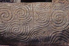
Megalithic art from Newgrange showing an early interest in curves

Interest in curves began long before they were the subject of mathematical study. This can be seen in numerous examples of their decorative use in art and on everyday objects dating back to prehistoric
times.^[1] Curves, or at least their graphical representations, are simple to create, for example by a stick in the sand on a beach.

Historically, the term "line" was used in place of the more modern term "curve". Hence the phrases "straight line" and "right line" were used to distinguish what are today called lines from "curved lines". For example, in Book I of Euclid's Elements, a line is defined as a "breadthless length" (Def. 2), while a straight line is defined as "a line that lies evenly with the points on itself" (Def. 4). Euclid's idea of a line is perhaps clarified by the statement "The extremities of a line are points," (Def. 3).^[2] Later commentators further classified lines according to various schemes. For example:^[3]

• Composite lines (lines forming an angle)


• Incomposite lines
  
  
  
  • Determinate (lines that do not extend indefinitely, such as the circle)
  
  
  • Indeterminate (lines that extend indefinitely, such as the straight line and the parabola)
  
  
  
  

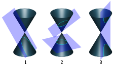
The curves created by slicing a cone (conic sections) were among the curves studied in ancient Greece.

The Greek geometers had studied many other kinds of curves. One reason was their interest in solving geometrical problems that could not be solved using standard compass and straightedge construction.
These curves include:

• The conic sections, deeply studied by Apollonius of Perga
  


• The cissoid of Diocles, studied by Diocles and used as a method to double the cube.^[4]
  


• The conchoid of Nicomedes, studied by Nicomedes as a method to both double the cube and to trisect an angle.^[5]
  


• The Archimedean spiral, studied by Archimedes as a method to trisect an angle and square the circle.^[6]
  


• The spiric sections, sections of tori studied by Perseus as sections of cones had been studied by Apollonius.

Analytic geometry allowed curves, such as the Folium of Descartes, to be defined using equations instead of geometrical construction.

A fundamental advance in the theory of curves was the advent of analytic geometry in the seventeenth century. This enabled a curve to be described using an equation rather than an elaborate geometrical construction. This not only allowed new curves to be defined and studied, but it enabled a formal distinction to be made between curves that can be defined using algebraic equations, algebraic curves, and those that cannot, transcendental curves. Previously, curves had been described as "geometrical" or "mechanical" according to how they were, or supposedly could be, generated.^[1]

Conic sections were applied in astronomy by Kepler.
Newton also worked on an early example in the calculus of variations. Solutions to variational problems, such as the brachistochrone and tautochrone questions, introduced properties of curves in new ways (in this case, the cycloid). The catenary gets its name as the solution to the problem of a hanging chain, the sort of question that became routinely accessible by means of differential calculus.

In the eighteenth century came the beginnings of the theory of plane algebraic curves, in general. Newton had studied the cubic curves, in the general description of the real points into 'ovals'. The statement of Bézout's theorem showed a number of aspects which were not directly accessible to the geometry of the time, to do with singular points and complex solutions.

Since the nineteenth century there has not been a separate theory of curves, but rather the appearance of curves as the one-dimensional aspect of projective geometry, and differential geometry; and later topology, when for example the Jordan curve theorem was understood to lie quite deep, as well as being required in complex analysis. The era of the space-filling curves finally provoked the modern definitions of curve.

Definition

Boundaries of hyperbolic components of Mandelbrot set as closed curves

In general, a curve is defined through a continuous function γ:I→X{displaystyle gamma colon Irightarrow X} from an interval I of the real numbers into a topological space X. Depending on the context, it is either γ{displaystyle gamma } or its image γ(I){displaystyle gamma (I)} which is called a curve.

In general topology, when non-differentiable functions are considered, it is the map γ{displaystyle gamma }, which is called a curve, because its image may look very differently from what is commonly called a curve. For example, the image of the Peano curve completely fills the square. On the other hand, when one considers curves defined by a differentiable function (or, at least, a piecewise differentiable function), this is commonly the image of the function which is called a curve.

• The curve is said to be simple, or a Jordan arc, if γ{displaystyle gamma } is injective, i.e. if for all x{displaystyle x}, y{displaystyle y} in I{displaystyle I}, we have γ(x)=γ(y){displaystyle gamma (x)=gamma (y)} implies x=y{displaystyle x=y}. If I{displaystyle I} is a closed bounded interval [a,b]{displaystyle [a,b]}, we also allow the possibility γ(a)=γ(b){displaystyle gamma (a)=gamma (b)} (this convention makes it possible to talk about "closed" simple curves, see below). In other words, this curve "does not cross itself and has no missing points".^[7]
  


• If γ(x)=γ(y){displaystyle gamma (x)=gamma (y)} for some x≠y{displaystyle xneq y} (other than the extremities of I{displaystyle I}), then γ(x){displaystyle gamma (x)} is called a double (or multiple) point of the curve. This is a special case of a singular point of a curve.


• A curve γ{displaystyle gamma } is said to be closed or a loop if I=[a,b]{displaystyle I=[a,b]} and if γ(a)=γ(b){displaystyle gamma (a)=gamma (b)}. A closed curve is thus the image of a continuous mapping of the circle S1{displaystyle S^{1}}; a simple closed curve is also called a Jordan curve. The Jordan curve theorem states that such curves divide the plane into an "interior" and an "exterior".

A plane curve is a curve for which X{displaystyle X} is the Euclidean plane—these are the examples first encountered—or in some cases the projective plane. A space curve is a curve for which X{displaystyle X} is of three dimensions, usually Euclidean space; a skew curve is a space curve which lies in no plane. These definitions of plane, space and skew curves apply also to real algebraic curves, although the above definition of a curve does not apply (a real algebraic curve may be disconnected).

This definition of curve captures our intuitive notion of a curve as a connected, continuous geometric figure that is "like" a line, without thickness and drawn without interruption, although it also includes figures that can hardly be called curves in common usage. For example, the image of a curve can cover a square in the plane (space-filling curve). The image of simple plane curve can have Hausdorff dimension bigger than one (see Koch snowflake) and even positive Lebesgue measure^[8] (the last example can be obtained by small variation of the Peano curve construction). The dragon curve is another unusual example.

Differentiable curve

Roughly speaking a differentiable curve is a curve that is defined as being locally the image of an injective differentiable function γ:I→X{displaystyle gamma colon Irightarrow X} from an interval I of the real numbers into a differentiable manifold X, often Rn.{displaystyle mathbb {R} ^{n}.}

More precisely, a differentiable curve is a subset C of X where every point of C has a neighborhood U such that C∩U{displaystyle Ccap U} is diffeomorphic to an interval of the real numbers. In other words, a differentiable curve is a differentiable manifold of dimension one.

Length of a curve

If X=Rn{displaystyle X=mathbb {R} ^{n}} is the n{displaystyle n}-dimensional Euclidean space, and if γ:[a,b]→Rn{displaystyle gamma :[a,b]to mathbb {R} ^{n}} is an injective and continuously differentiable function, then the length of γ{displaystyle gamma } is defined as the quantity

Length⁡(γ) =df ∫ab|γ′(t)| dt.{displaystyle operatorname {Length} (gamma )~{stackrel {text{df}}{=}}~int _{a}^{b}|gamma ,'(t)|~mathrm {d} {t}.}

The length of a curve is independent of the parametrization γ{displaystyle gamma }.

In particular, the length s{displaystyle s} of the graph of a continuously differentiable function y=f(x){displaystyle y=f(x)} defined on a closed interval [a,b]{displaystyle [a,b]} is

s=∫ab1+[f′(x)]2 dx.{displaystyle s=int _{a}^{b}{sqrt {1+[f'(x)]^{2}}}~mathrm {d} {x}.}

More generally, if X{displaystyle X} is a metric space with metric d{displaystyle d}, then we can define the length of a curve γ:[a,b]→X{displaystyle gamma :[a,b]to X} by

Length⁡(γ) =df sup({∑i=1nd(γ(ti),γ(ti−1)) | n∈N and a=t0<t1<…<tn=b}),{displaystyle operatorname {Length} (gamma )~{stackrel {text{df}}{=}}~sup !left(left{sum _{i=1}^{n}d(gamma (t_{i}),gamma (t_{i-1}))~{Bigg |}~nin mathbb {N} ~{text{and}}~a=t_{0}<t_{1}<ldots <t_{n}=bright}right),}

where the supremum is taken over all n∈N{displaystyle nin mathbb {N} } and all partitions t0<t1<…<tn{displaystyle t_{0}<t_{1}<ldots <t_{n}} of [a,b]{displaystyle [a,b]}.

A rectifiable curve is a curve with finite length. A curve γ:[a,b]→X{displaystyle gamma :[a,b]to X} is called natural (or unit-speed or parametrized by arc length) if for any t1,t2∈[a,b]{displaystyle t_{1},t_{2}in [a,b]} such that t1≤t2{displaystyle t_{1}leq t_{2}}, we have

Length(γ|[t1,t2])=t2−t1.{displaystyle operatorname {Length} !left(gamma |_{[t_{1},t_{2}]}right)=t_{2}-t_{1}.}

If γ:[a,b]→X{displaystyle gamma :[a,b]to X} is a Lipschitz-continuous function, then it is automatically rectifiable. Moreover, in this case, one can define the speed (or metric derivative) of γ{displaystyle gamma } at t∈[a,b]{displaystyle tin [a,b]} as

Speedγ(t) =df lim sup[a,b]∋s→td(γ(s),γ(t))|s−t|{displaystyle {operatorname {Speed} _{gamma }}(t)~{stackrel {text{df}}{=}}~limsup _{[a,b]ni sto t}{frac {d(gamma (s),gamma (t))}{|s-t|}}}

and then show that

Length⁡(γ)=∫abSpeedγ(t) dt.{displaystyle operatorname {Length} (gamma )=int _{a}^{b}{operatorname {Speed} _{gamma }}(t)~mathrm {d} {t}.}

Differential geometry

While the first examples of curves that are met are mostly plane curves (that is, in everyday words, curved lines in two-dimensional space), there are obvious examples such as the helix which exist naturally in three dimensions. The needs of geometry, and also for example classical mechanics are to have a notion of curve in space of any number of dimensions. In general relativity, a world line is a curve in spacetime.

If X{displaystyle X} is a differentiable manifold, then we can define the notion of differentiable curve in X{displaystyle X}. This general idea is enough to cover many of the applications of curves in mathematics. From a local point of view one can take X{displaystyle X} to be Euclidean space. On the other hand, it is useful to be more general, in that (for example) it is possible to define the tangent vectors to X{displaystyle X} by means of this notion of curve.

If X{displaystyle X} is a smooth manifold, a smooth curve in X{displaystyle X} is a smooth map

γ:I→X{displaystyle gamma colon Irightarrow X}.

This is a basic notion. There are less and more restricted ideas, too. If X{displaystyle X} is a Ck{displaystyle C^{k}} manifold (i.e., a manifold whose charts are k{displaystyle k} times continuously differentiable), then a Ck{displaystyle C^{k}} curve in X{displaystyle X} is such a curve which is only assumed to be Ck{displaystyle C^{k}} (i.e. k{displaystyle k} times continuously differentiable). If X{displaystyle X} is an analytic manifold (i.e. infinitely differentiable and charts are expressible as power series), and γ{displaystyle gamma } is an analytic map, then γ{displaystyle gamma } is said to be an analytic curve.

A differentiable curve is said to be regular if its derivative never vanishes. (In words, a regular curve never slows to a stop or backtracks on itself.) Two Ck{displaystyle C^{k}} differentiable curves

γ1:I→X{displaystyle gamma _{1}colon Irightarrow X} and

γ2:J→X{displaystyle gamma _{2}colon Jrightarrow X}

are said to be equivalent if there is a bijective Ck{displaystyle C^{k}} map

p:J→I{displaystyle pcolon Jrightarrow I}

such that the inverse map

p−1:I→J{displaystyle p^{-1}colon Irightarrow J}

is also Ck{displaystyle C^{k}}, and

γ2(t)=γ1(p(t)){displaystyle gamma _{2}(t)=gamma _{1}(p(t))}

for all t{displaystyle t}. The map γ2{displaystyle gamma _{2}} is called a reparametrisation of γ1{displaystyle gamma _{1}}; and this makes an equivalence relation on the set of all Ck{displaystyle C^{k}} differentiable curves in X{displaystyle X}. A Ck{displaystyle C^{k}} arc is an equivalence class of Ck{displaystyle C^{k}} curves under the relation of reparametrisation.

Algebraic curve

Algebraic curves are the curves considered in algebraic geometry. A plane algebraic curve is the set of the points of coordinates x, y such that f(x, y) = 0, where f is a polynomial in two variables defined over some field F. Algebraic geometry normally looks not only on points with coordinates in F but on all the points with coordinates in an algebraically closed field K. If C is a curve defined by a polynomial f with coefficients in F, the curve is said to be defined over F. The points of the curve C with coordinates in a field G are said to be rational over G and can be denoted C(G)). When G is the field of the rational numbers, one simply talks of rational points. For example, Fermat's Last Theorem may be restated as: For n > 2, every rational point of the Fermat curve of degree n has a zero coordinate.

Algebraic curves can also be space curves, or curves in a space of higher dimension, say n. They are defined as algebraic varieties of dimension one. They may be obtained as the common solutions of at least n–1 polynomial equations in n variables. If n–1 polynomials are sufficient to define a curve in a space of dimension n, the curve is said to be a complete intersection. By eliminating variables (by any tool of elimination theory), an algebraic curve may be projected onto a plane algebraic curve, which however may introduce new singularities such as cusps or double points.

A plane curve may also be completed in a curve in the projective plane: if a curve is defined by a polynomial f of total degree d, then w^df(u/w, v/w) simplifies to a homogeneous polynomial g(u, v, w) of degree d. The values of u, v, w such that g(u, v, w) = 0 are the homogeneous coordinates of the points of the completion of the curve in the projective plane and the points of the initial curve are those such w is not zero. An example is the Fermat curve uⁿ + vⁿ = wⁿ, which has an affine form xⁿ + yⁿ = 1. A similar process of homogenization may be defined for curves in higher dimensional spaces

Important examples of algebraic curves are the conics, which are nonsingular curves of degree two and genus zero, and elliptic curves, which are nonsingular curves of genus one studied in number theory and which have important applications to cryptography. Because algebraic curves in fields of characteristic zero are most often studied over the complex numbers, algebraic curves in algebraic geometry may be considered as real surfaces. In particular, the nonsingular complex projective algebraic curves are called Riemann surfaces.

See also

Notes

References

• 
  A.S. Parkhomenko (2001) [1994], "Line (curve)", in Hazewinkel, Michiel, Encyclopedia of Mathematics, Springer Science+Business Media B.V. / Kluwer Academic Publishers, ISBN 978-1-55608-010-4
  


• 
  B.I. Golubov (2001) [1994], "Rectifiable curve", in Hazewinkel, Michiel, Encyclopedia of Mathematics, Springer Science+Business Media B.V. / Kluwer Academic Publishers, ISBN 978-1-55608-010-4
  


• 
  Euclid, commentary and trans. by T. L. Heath Elements Vol. 1 (1908 Cambridge) Google Books
  


• E. H. Lockwood A Book of Curves (1961 Cambridge)

External links

Wikimedia Commons has media related to Curves.

• 
  Famous Curves Index, School of Mathematics and Statistics, University of St Andrews, Scotland


• 
  Mathematical curves A collection of 874 two-dimensional mathematical curves


• Gallery of Space Curves Made from Circles, includes animations by Peter Moses


• Gallery of Bishop Curves and Other Spherical Curves, includes animations by Peter Moses


• The Encyclopedia of Mathematics article on lines.


• The Manifold Atlas page on 1-manifolds.